Setup
Create directory structure and clone repo
(Working directory on EBI cluster: /hps/research1/birney/users/ian/mikk_paper)
# move to working directory
cd /your/working/directory
# clone git repository
git clone https://github.com/Ian-Brettell/mikk_genome.git
Create conda evironment
conda env create \
  -n mikk_env \
  -f mikk_genome/code/config/conda_env.yml

conda activate mikk_env
Setup R
# Load required libraries
require(here)
source(here::here("code/scripts/ld_decay/source.R"))
Copy MIKK panel VCF into working directory
(See supplementary material for how VCF was generated.)
# create directory for VCFs
mkdir vcfs

# Copy into working directory
cp /nfs/research1/birney/projects/medaka/inbred_panel/medaka-alignments-release-94/vcf/medaka_inbred_panel_ensembl_new_reference_release_94.vcf* vcfs
Key-value file for cram ID to line ID
mikk_genome/data/20200206_cram_id_to_line_id.txt
Remove sibling lines and replicates
Full list of 80 extant MIKK panel lines: mikk_genome/data/20200210_panel_lines_full.txt
Note: Line 130-2 is missing from the MIKK panel VCF.
Identify sibling lines
cat mikk_genome/data/20200210_panel_lines_full.txt | cut -f1 -d"-" | sort | uniq -d
- 106
- 11
- 117
- 131
- 132
- 135
- 14
- 140
- 23
- 39
- 4
- 40
- 59
- 69
- 72
- 80
Only keep first sibling line ( suffix _1); manually remove all others and write list of non-sibling lines to here: mikk_genome/data/20200227_panel_lines_no-sibs.txt. 64 lines total.
Excluded sibling lines here: mikk_genome/data/20200227_panel_lines_excluded.txt. 16 lines total.
Replace all dashes with underscores to match mikk_genome/data/20200206_cram_id_to_line_id.txt key file
sed 's/-/_/g' mikk_genome/data/20200227_panel_lines_no-sibs.txt \
  > mikk_genome/data/20200227_panel_lines_no-sibs_us.txt
Extract the lines to keep from the key file.
awk  'FNR==NR {f1[$0]; next} $2 in f1' \
  mikk_genome/data/20200227_panel_lines_no-sibs_us.txt \
  mikk_genome/data/20200206_cram_id_to_line_id.txt \
    > mikk_genome/data/20200227_cram2line_no-sibs.txt
Has 66 lines instead of 63 (64 lines minus 130-2, which isn’t in the VCF), so there must be replicates Find out which ones:
cat mikk_genome/data/20200227_cram2line_no-sibs.txt | cut -f2 | cut -f1 -d"_" | sort | uniq -d
32 71 84
Manually removed duplicate lines (mikk_genome/data/20200227_duplicates_excluded.txt):
- 24271_7#5 32_2
- 24271_8#4 71_1
- 24259_1#1 84_2
Final no-sibling-lines CRAM-to-lineID key file: mikk_genome/data/20200227_cram2line_no-sibs.txt
Create MIKK panel VCF with no sibling lines
# create no-sibs file with CRAM ID only
cut -f1 mikk_genome/data/20200227_cram2line_no-sibs.txt \
  > mikk_genome/data/20200227_cram2line_no-sibs_cram-only.txt

# make new VCF having filtered out non-MIKK and sibling lines
bcftools view \
  --output-file vcfs/panel_no-sibs.vcf \
  --samples-file mikk_genome/data/20200227_cram2line_no-sibs_cram-only.txt \
  vcfs/medaka_inbred_panel_ensembl_new_reference_release_94.vcf

# recode with line IDs
bcftools reheader \
  --output vcfs/panel_no-sibs_line-ids.vcf \
  --samples mikk_genome/data/20200227_cram2line_no-sibs.txt \
  vcfs/panel_no-sibs.vcf

# compress
bcftools view \
  --output-type z \
  --output-file vcfs/panel_no-sibs_line-ids.vcf.gz \
  vcfs/panel_no-sibs_line-ids.vcf

# index
bcftools index \
  --tbi \
  vcfs/panel_no-sibs_line-ids.vcf.gz

# get stats
mkdir stats

bcftools stats \
  vcfs/panel_no-sibs_line-ids.vcf.gz \
  > stats/20200305_panel_no-sibs.txt

## get basic counts
grep "^SN" stats/20200305_panel_no-sibs.txt
Make a version with no missing variants
vcftools \
  --gzvcf vcfs/panel_no-sibs_line-ids.vcf.gz \
  --max-missing 1 \
  --recode \
  --stdout > vcfs/panel_no-sibs_line-ids_no-missing.vcf

# compress
bcftools view \
  --output-type z \
  --output-file vcfs/panel_no-sibs_line-ids_no-missing.vcf.gz \
  vcfs/panel_no-sibs_line-ids_no-missing.vcf

# create index
bcftools index \
  --tbi vcfs/panel_no-sibs_line-ids_no-missing.vcf.gz

# get stats
bcftools stats \
  vcfs/panel_no-sibs_line-ids_no-missing.vcf.gz \
  > stats/20200305_panel_no-sibs_no-missing.txt

# get basic counts
grep "^SN" stats/20200305_panel_no-sibs_no-missing.txt
Generate Haploview plots
Create plink dataset from no-sib-lines, no-missing VCF
mkdir plink/20200716_panel_no-sibs_line-ids_no-missing

# make BED
plink \
  --vcf vcfs/panel_no-sibs_line-ids_no-missing.vcf.gz \
  --make-bed \
  --double-id \
  --snps-only \
  --biallelic-only \
  --chr-set 24 no-xy \
  --chr 1-24 \
  --out plink/20200716_panel_no-sibs_line-ids_no-missing/20200716

# recode for 012 transposed
plink \
  --bfile plink/20200716_panel_no-sibs_line-ids_no-missing/20200716 \
  --recode A-transpose \
  --out plink/20200716_panel_no-sibs_line-ids_no-missing/20200716_recode012
# creates plink/20200716_panel_no-sibs_line-ids_no-missing/20200716_recode012.traw
Create BED sets filtered for MAF > 0.03, 0.05 and 0.10
maf_thresholds=$( echo 0.03 0.05 0.10 )

# Make new BEDs
for i in $maf_thresholds ; do
  # make directory
  new_path=plink/20200716_panel_no-sibs_line-ids_no-missing/20200803_maf-$i ;
  # make directory
  if [ ! -d "$new_path" ]; then
    mkdir $new_path;
  fi
  # make BED set
  plink \
    --bfile plink/20200716_panel_no-sibs_line-ids_no-missing/20200716 \
    --make-bed \
    --double-id \
    --chr-set 24 no-xy \
    --maf $i \
    --out $new_path/20200803
done
Recode for Haploview
# Create output directory
mkdir plink/20200716_panel_no-sibs_line-ids_no-missing/20200803_hv_thinned

hv_thinned_path=plink/20200716_panel_no-sibs_line-ids_no-missing/20200803_hv_thinned

# Recode
for i in $maf_thresholds ; do
  new_path=$hv_thinned_path/$i ;
  # make directory
  if [ ! -d "$new_path" ]; then
    mkdir $new_path;
  fi
  # recode
  for j in $(seq 1 24); do
    plink \
      --bfile plink/20200716_panel_no-sibs_line-ids_no-missing/20200803_maf-$i/20200803 \
      --recode HV-1chr \
      --double-id \
      --chr-set 24 no-xy \
      --chr $j \
      --allele1234 \
      --thin-count 3000 \
      --out $hv_thinned_path/$i/20200803_chr-$j;
  done;
done

# Edit .ped files to remove asterisks
for i in $maf_thresholds ; do
  for j in $(find $hv_thinned_path/$i/20200803_chr-*.ped); do
    sed -i 's/\*/0/g' $j;
  done;
done

# Edit .info files to make the SNP's bp position its ID
for i in $maf_thresholds; do
  for j in $(find $hv_thinned_path/$i/20200803_chr*.info); do
    outname=$(echo $j\_with-id);
    awk -v OFS="\t" {'print $2,$2'} $j > $outname;
  done;
done
Plot
NOTE: This code requires Haploview, which you will need to install on your system: https://www.broadinstitute.org/haploview/haploview
hv_path=/nfs/software/birney/Haploview.jar # edit to your Haploview path

mkdir plots/20200803_ld_thinned/

for i in $maf_thresholds; do
  # set output directory
  new_path=plots/20200803_ld_thinned/$i ;
  # make directory
  if [ ! -d "$new_path" ]; then
    mkdir $new_path;
  fi
  for j in $(seq 1 24); do
    bsub -M 20000 -o log/20200803_hv_$i\_$j.out -e log/20200803_hv_$i\_$j.err \
    "java -Xms18G -Xmx18G -jar $hv_path \
      -memory 18000 \
      -pedfile $hv_thinned_path/$i/20200803_chr-$j.ped  \
      -info $hv_thinned_path/$i/20200803_chr-$j.info_with-id \
      -maxDistance 1000 \
      -ldcolorscheme DEFAULT \
      -ldvalues RSQ \
      -minMAF $i \
      -nogui \
      -svg \
      -out $new_path/$j";
  done;
done
These svg files can be converted to pdf using:
The full Haploview LD plots are available in the Supplementary Material.
By inspecting these LD plots at the MAF > 0.05 level, we discovered the following LD blocks worthy of further investigation:
- 5:28181970-28970558 (788 Kb)
- 6:29398579-32246747 (2.85 Mb)
- 12:25336174-25384053 (48 Kb)
- 14:12490842-12947083 (456 Kb)
- 17:15557892-19561518 (4 Mb)
- 21:6710074-7880374 (1.17 Mb)
See zoomed plots here:
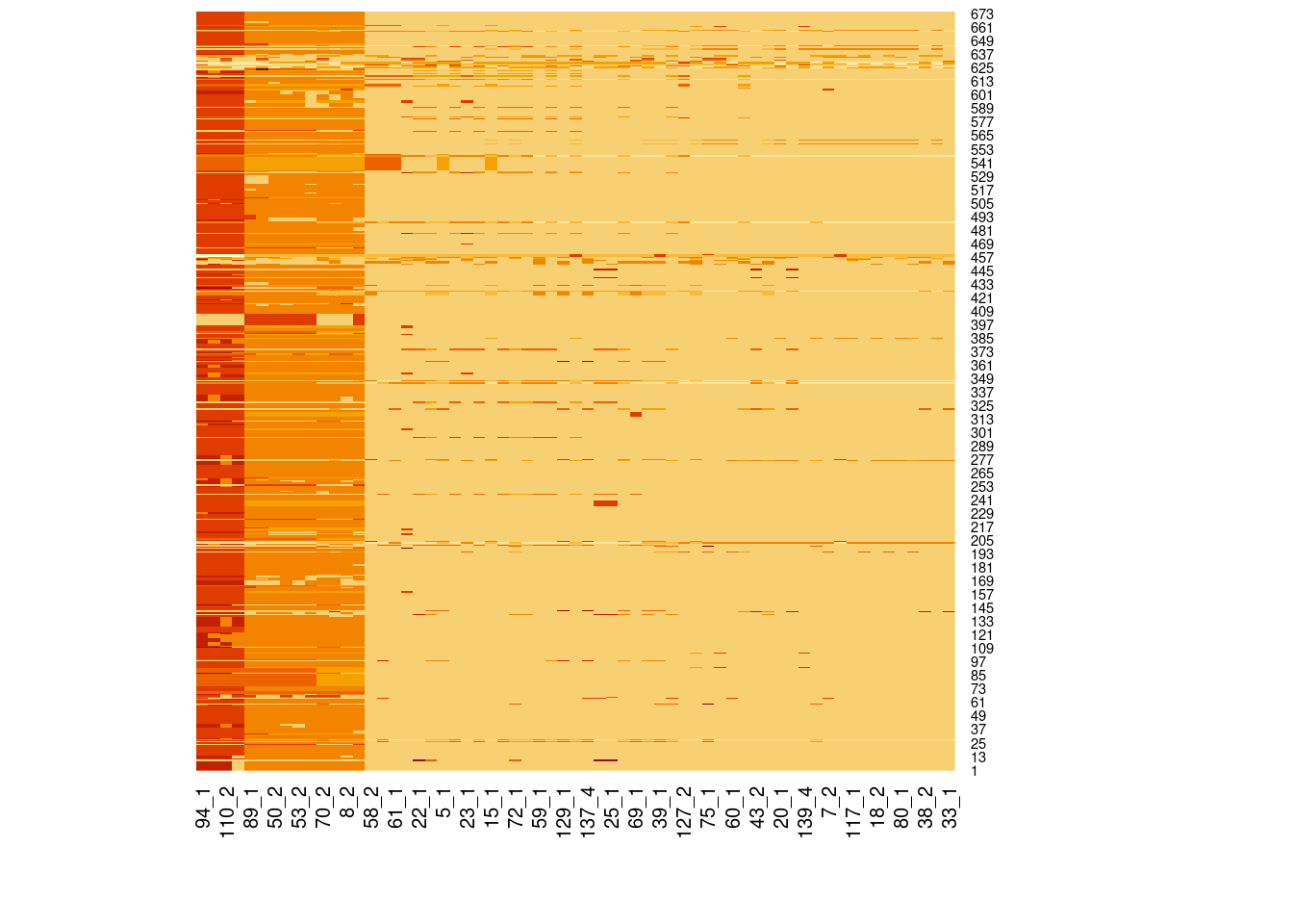
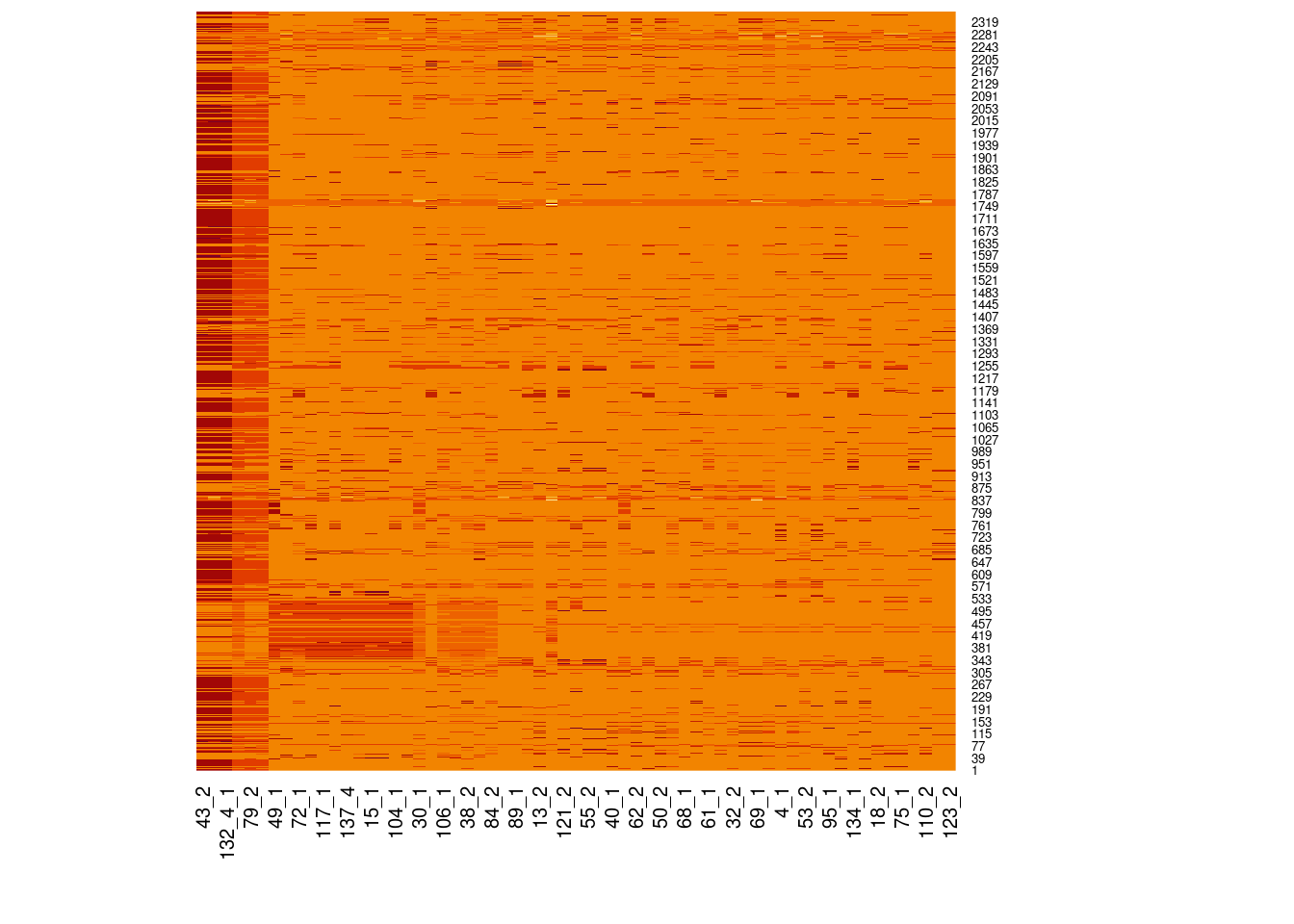
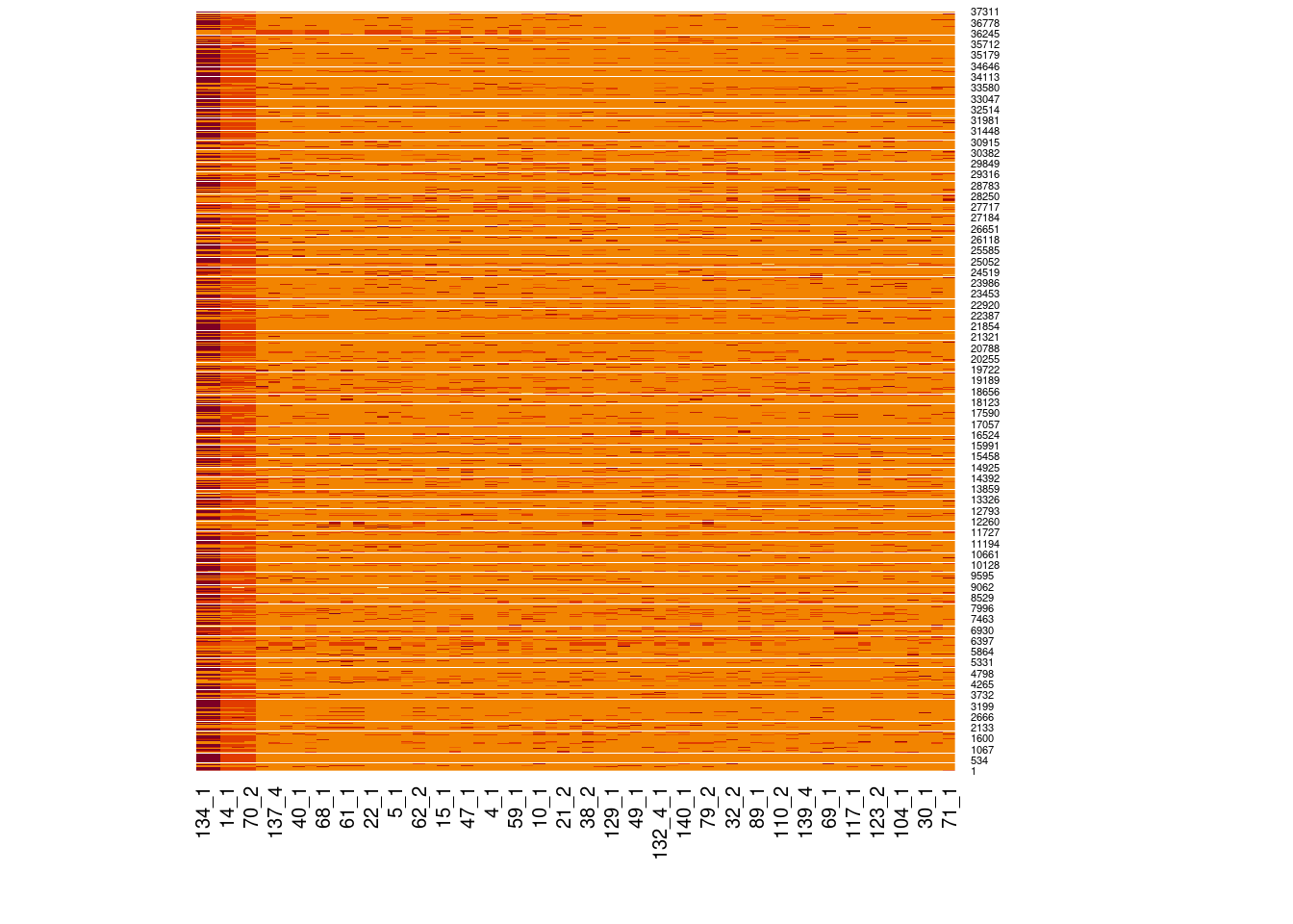
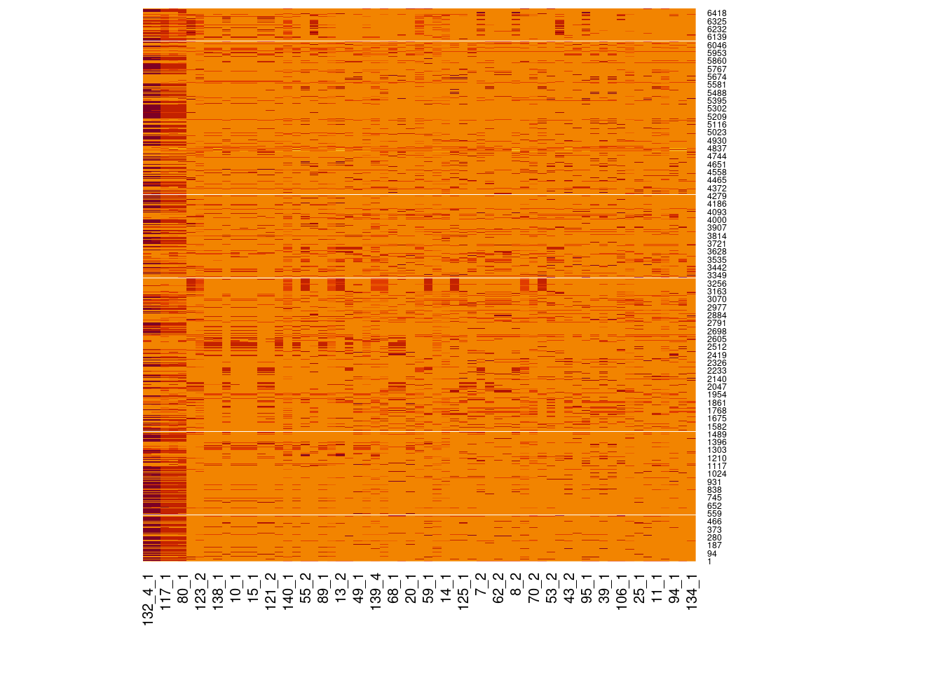
Genotype heatmaps for high-LD regions
See which lines are causing the high-LD regions at the MAF > 0.05 threshold (i.e. from a sample of 63 diploid individuals, variants with an allele count (AC) of at least 7).
Read data into BED matrix into R
# Read in BED matrix
mikk_full <- gaston::read.bed.matrix(file.path(lts_dir, "plink/20200716_panel_no-sibs_line-ids_no-missing/20200716"),
                                     rds = NULL)

# Read in genotypes file
mikk_geno <- readr::read_tsv(file = file.path(lts_dir, "plink/20200716_panel_no-sibs_line-ids_no-missing/20200716_recode012.traw"),
                             progress = T,
                             col_names = T)

# rename IDs
colnames(mikk_geno)[7:length(colnames(mikk_geno))] <- mikk_full@ped$id
Extract target regions and build into list
# get coordinates
high_ld_chrs <- c(5, 6, 12, 14, 17, 21)
high_ld_start <- c(28385805, 29608514, 25340000, 12584614, 15559963, 6800261)
high_ld_end <- c(28798048, 32212235, 25372985, 12861147, 19553529, 7760258)

# build into list
counter <- 0
high_ld_lst <- lapply(high_ld_chrs, function(x){
  counter <<- counter + 1
  x <- list("chr" = x,
            "start" = high_ld_start[counter],
            "end" = high_ld_end[counter])
  # find indexes for SNPs with MAF > 0.05
  x[["target_inds"]] <- which(mikk_full@snps$chr == x[["chr"]] &
                         dplyr::between(mikk_full@snps$pos, x[["start"]], x[["end"]]) &
                         mikk_full@snps$maf > 0.05)
  x[["target_snps"]] <- mikk_geno[x[["target_inds"]], ]
  # make matrix
  x[["geno_mat"]] <- as.matrix(x[["target_snps"]][, -(1:6)])
  return(x)
})
names(high_ld_lst) <- high_ld_chrs

# save to repo
saveRDS(high_ld_lst, file.path(lts_dir, "20200727_high_ld_list.rds"))
Plot
Genotypes were recoded to 0, 1, 2 for REF, HET, and HOM_ALT respectively.
Dark red = 2 Orange = 1 Yellow = 0
# Write function to create heatmap
get_heatmap = function(in_list){
  # Get order of samples
  sample_order = colnames(in_list[["target_snps"]])[-(1:6)]
  # Sort by count
  sorted_order = names(sort(colSums(in_list[["geno_mat"]]), decreasing = T))
  # Get re-ordered indein_listes
  new_ind = match(sorted_order, sample_order)
  # Plot
  heatmap(in_list[["geno_mat"]][, new_ind],
          Rowv = NA,
          Colv = NA,
          scale = "row",
          keep.dendro = F)
}
Chr 5
knitr::include_graphics(here::here("docs/plots/ld_decay/hv_5_28181970-28970558.png"))
x = high_ld_lst[["5"]]
get_heatmap(x)
Chr 6
knitr::include_graphics(here::here("docs/plots/ld_decay/hv_6_29398579-32246747.png"))
x = high_ld_lst[["6"]]
get_heatmap(x)
Chr 12
knitr::include_graphics(here::here("docs/plots/ld_decay/hv_12_25336174-25384053.png"))
x = high_ld_lst[["12"]]
get_heatmap(x)
Chr 14
knitr::include_graphics(here::here("docs/plots/ld_decay/hv_14_12490842-12947083.png"))
x = high_ld_lst[["14"]]
get_heatmap(x)
Chr 17
knitr::include_graphics(here::here("docs/plots/ld_decay/hv_17_15557892-19561518.png"))
x = high_ld_lst[["17"]]
get_heatmap(x)
Chr 21
knitr::include_graphics(here::here("docs/plots/ld_decay/hv_21_6710074-7880374.png"))
x = high_ld_lst[["21"]]
get_heatmap(x)
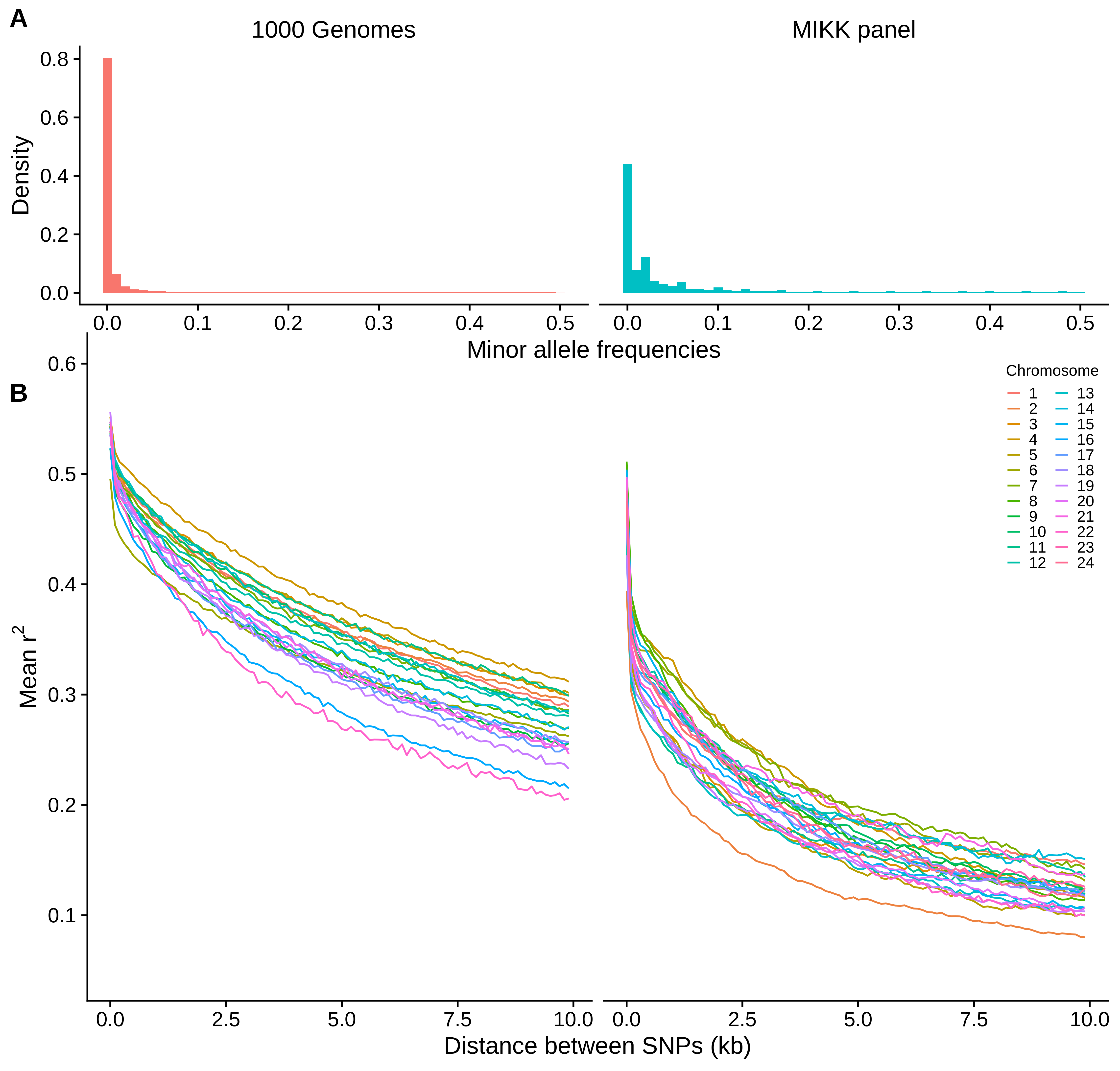
LD decay
We want to compare the rate at which LD decays with inter-SNP distance between the MIKK panel and humans. This will give an indication of the resolution at which one can map genetic traits using the MIKK panel, provided that at least two lines have the same variant of interest.
Obtain 1000 Genomes dataset
Download from FTP
cd vcfs

wget -r -p -k --no-parent -cut-dirs=5 ftp://ftp.1000genomes.ebi.ac.uk/vol1/ftp/release/20130502/
Put list of files into list
find vcfs/ftp.1000genomes.ebi.ac.uk/ALL.chr*.vcf.gz > mikk_genome/data/20200205_vcfs.list
Merge VCFs
# Remove MT and Y from list
sed -i '/MT/d' mikk_genome/data/20200205_vcfs.list

sed -i '/chrY/d' mikk_genome/data/20200205_vcfs.list

# run MergeVCFs
java -jar /nfs/software/birney/picard-2.9.0/picard.jar MergeVcfs \
  I=mikk_genome/data/20200205_vcfs.list \
  O=vcfs/1gk_all.vcf.gz
Get LD stats using Plink
# make BED
mkdir plink/20200727_mikk_no-missing_maf-0.05

plink \
  --vcf vcfs/panel_no-sibs_line-ids.vcf.gz \
  --make-bed \
  --double-id \
  --snps-only \
  --biallelic-only \
  --maf 0.05 \
  --geno 0 \
  --chr-set 24 no-xy \
  --out plink/20200727_mikk_no-missing_maf-0.05/20200727

# get LD stats for MIKK
mkdir ld/20200727_mikk_maf-0.10_window-50kb_no-missing/

for i in $(seq 1 24); do
  plink \
      --bfile plink/20200727_mikk_no-missing_maf-0.05/20200727 \
      --r2 \
      --ld-window 999999 \
      --ld-window-kb 50 \
      --ld-window-r2 0 \
      --chr-set 24 no-xy \
      --chr $i \
      --maf 0.10 \
      --out ld/20200727_mikk_maf-0.10_window-50kb_no-missing/$i;
done

# get LD stats for 1KG
mkdir ld/20200727_1kg_maf-0.10_window-50kb_no-missing/

for i in $(seq 1 22); do
  plink \
      --bfile plink/20200723_1gk_no-missing_maf-0.05/20200723 \
      --r2 \
      --ld-window 999999 \
      --ld-window-kb 50 \
      --ld-window-r2 0 \
      --chr $i \
      --maf 0.10 \
      --out ld/20200727_1kg_maf-0.10_window-50kb_no-missing/$i;
done

# do again with ld-window-kb 10 to get counts of comparisons for paper
# MIKK
mkdir ld/20200803_mikk_maf-0.10_window-10kb_no-missing/

for i in $(seq 1 24); do
  plink \
      --bfile plink/20200727_mikk_no-missing_maf-0.05/20200727 \
      --r2 \
      --ld-window 999999 \
      --ld-window-kb 10 \
      --ld-window-r2 0 \
      --chr-set 24 no-xy \
      --chr $i \
      --maf 0.10 \
      --out ld/20200803_mikk_maf-0.10_window-10kb_no-missing/$i;
done

# 1KG
mkdir ld/20200803_1kg_maf-0.10_window-10kb_no-missing/

for i in $(seq 1 22); do
  plink \
      --bfile plink/20200723_1gk_no-missing_maf-0.05/20200723 \
      --r2 \
      --ld-window 999999 \
      --ld-window-kb 10 \
      --ld-window-r2 0 \
      --chr $i \
      --maf 0.10 \
      --out ld/20200803_1kg_maf-0.10_window-10kb_no-missing/$i;
done

# Get total counts of pairwise comparisons:
wc -l ld/20200803_mikk_maf-0.10_window-10kb_no-missing/*.ld
# 204,152,898
wc -l ld/20200803_1kg_maf-0.10_window-10kb_no-missing/*.ld
Get mean LD within SNP-distance windows
0-10kb distance (main, MIKK v 1KG)
Rscript here: mikk_genome/code/scripts/20200727_r2_decay_mean_10kb-lim.R
MIKK
script=mikk_genome/code/scripts/20200727_r2_decay_mean_10kb-lim.R

mkdir ld/20200727_mean_r2_10kb-lim_mikk

for i in $(find ld/20200727_mikk_maf-0.10_window-50kb_no-missing/*.ld); do
  name=$(basename $i | cut -f1 -d".") ;
  out_dir=ld/20200727_mean_r2_10kb-lim_mikk ;
  bsub \
    -M 10000 \
    -o log/20200727_$name\_mean-r2_1kb-max.out \
    -e log/20200727_$name\_mean-r2_1kb-max.err \
    "Rscript --vanilla \
      $script \
      $i \
      $out_dir";
done
1KG
mkdir ld/20200727_mean_r2_10kb-lim_1kg

for i in $(find ld/20200727_1kg_maf-0.10_window-50kb_no-missing/*.ld); do
  name=$(basename $i | cut -f1 -d".") ;
  out_dir=ld/20200727_mean_r2_10kb-lim_1kg ;
  bsub \
    -M 30000 \
    -o log/20200727_$name\_mean-r2_10kb-max.out \
    -e log/20200727_$name\_mean-r2_10kb-max.err \
    "Rscript --vanilla \
      $script \
      $i \
      $out_dir";
done
0-1kb distance (inset, MIKK only)
Rscript: mikk_genome/code/scripts/20200803_r2_decay_mean_1gk_1kb-lim.R
mkdir ld/20200803_mean_r2_1kb-lim_mikk

out_dir=ld/20200803_mean_r2_1kb-lim_mikk
script=mikk_genome/code/scripts/20200803_r2_decay_mean_1gk_1kb-lim.R

for i in $(find ld/20200727_mikk_maf-0.10_window-50kb_no-missing/*ld); do
  name=$(basename $i | cut -f1 -d".");
  bsub \
    -M 30000 \
    -o log/20200803_$name\_mean-r2_1kb-max.out \
    -e log/20200803_$name\_mean-r2_1kb-max.err \
    "Rscript --vanilla \
      $script \
      $i \
      $out_dir";
done
Create LD plots in R
Main
Read in and process data
# Setup
require(here)
source(here::here("code", "scripts", "ld_decay", "source.R"))

# Create function to read in data and bind into single DF

read_n_bind = function(data_path_pref, dataset){
  # Set path
  path = paste(data_path_pref, dataset, sep = "")

  # Read in data
  data_files <- list.files(path,
                           full.names = T)
  data_files_trunc <- list.files(path)
  data_files_trunc <- gsub(".txt", "", data_files_trunc)

  data_list <- lapply(data_files, function(data_file){
    df <- read.delim(data_file,
                     sep = "\t",
                     header = T)
    return(df)
  })
  names(data_list) <- as.integer(data_files_trunc)

  # reorder
  data_list <- data_list[order(as.integer(names(data_list)))]

  # bind into DF
  out_df = dplyr::bind_rows(data_list, .id = "chr")
  out_df$chr <- factor(out_df$chr, levels = seq(1, 24))

  # get kb measure
  out_df$bin_bdr_kb <- out_df$bin_bdr / 1000

  return(out_df)
}

# Run over both datasets
datasets = c("mikk", "1kg")
final_lst = lapply(datasets, function(x) read_n_bind("ld/20200727_mean_r2_10kb-lim_", x))
names(final_lst) = datasets

# Combine into single DF
r2_final_df <- dplyr::bind_rows(final_lst, .id = "dataset")
# Write table to repo
write.table(r2_final_df,
            file = here::here("mikk_genome", "data", "20200803_r2_10kb-lim.csv"),
            quote = F, sep = ",", row.names = F, col.names = T)
Plot
# Tidy data for final plot
r2_final_df$chr = factor(r2_final_df$chr, levels = seq(1, 24))
r2_final_df$dataset = toupper(r2_final_df$dataset)

# Plot
r2_plot_main = r2_final_df %>% ggplot() +
  geom_line(aes(bin_bdr_kb, mean, colour = chr)) +
  theme_cowplot() +
  xlab("Distance between SNPs (kb)") +
  ylab(bquote(.("Mean r")^2)) +
  facet_wrap(~dataset, nrow = 1, ncol = 2) +
  theme(panel.grid = element_blank(),
        strip.background = element_blank(),
        legend.position = c(0.9, .8)) +
  labs(colour = "Chromosome") +
  scale_y_continuous(breaks = c(0.1, 0.2, 0.3, 0.4, 0.5, 0.6),
                     limits = c(0.05, 0.6))

#r2_plot_main
## Warning in if (robust_nchar(axisTitleText) > 0) {: the condition has length > 1 and only the first element will be used
## Warning in if (robust_nchar(axisTitleText) > 0) {: the condition has length > 1 and only the first element will be used
<<<<<<< HEAD
=======
>>>>>>> 1f72b2c38317bbf9e22e15671a199f851eaded2e
# Save plot to repo
ggsave(filename = paste("20200803_mean-r2_10kb-lim_1KGvMIKK_single", ".svg", sep = ""),
       plot = r2_plot_main,
       device = "svg",
       path = here::here("plots", "ld_decay"),
       width = 25,
       height = 13,
       units = "cm")
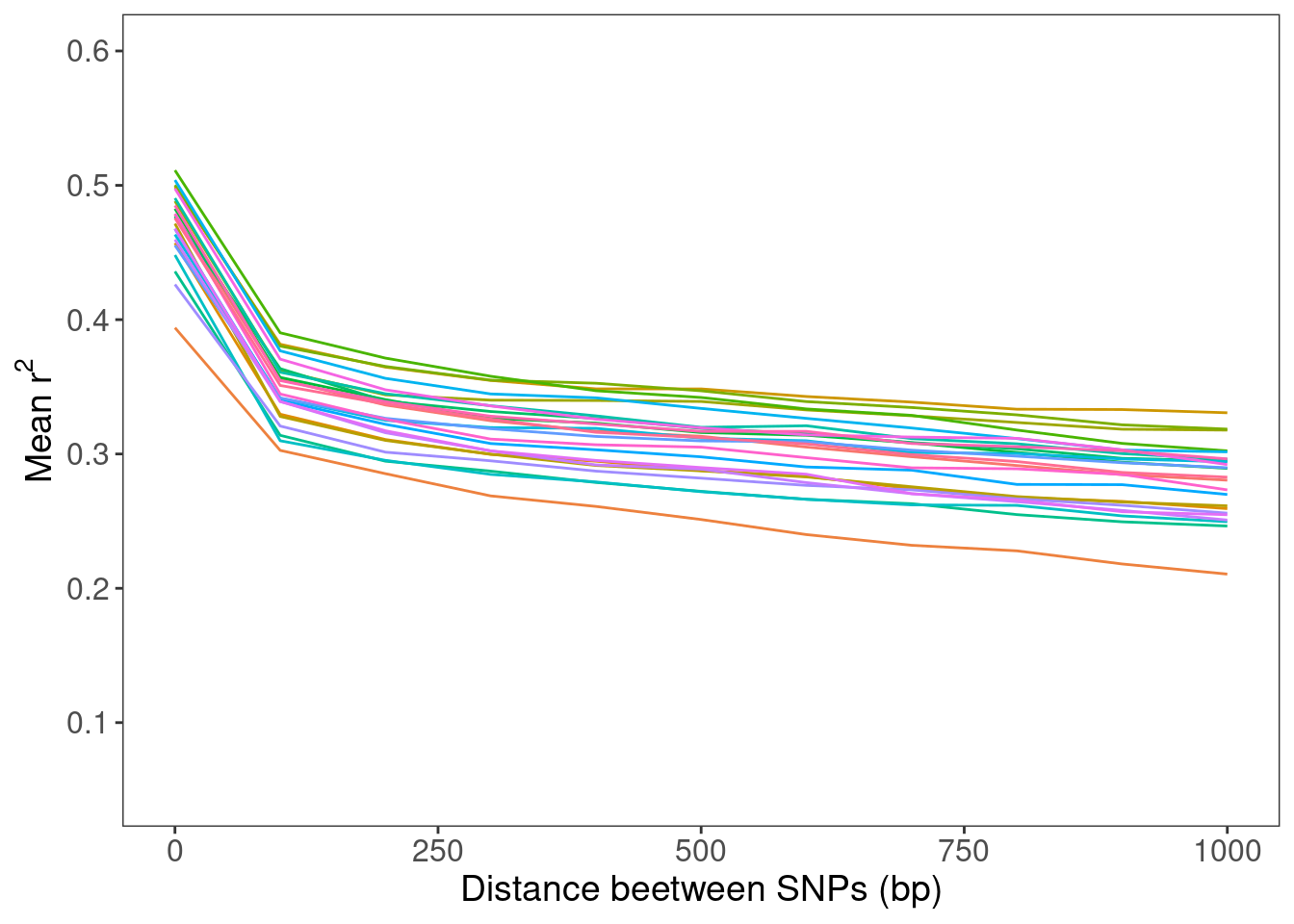
Inset
100-bp windows
# Read in data
r2_df_1kb_mikk = read_n_bind("ld/20200803_mean_r2_1kb-lim_", "mikk")
# Write table to repo
write.table(r2_df_1kb_mikk,
            file = here::here("mikk_genome", "data", "20200803_r2_1kb-lim_mikk.csv"),
            quote = F, sep = ",", row.names = F, col.names = T)
# Process for plotting
r2_df_1kb_mikk$chr <- factor(r2_df_1kb_mikk$chr, levels = seq(1, 24))
# Plot
r2_1kb_mikk = r2_df_1kb_mikk %>% ggplot() +
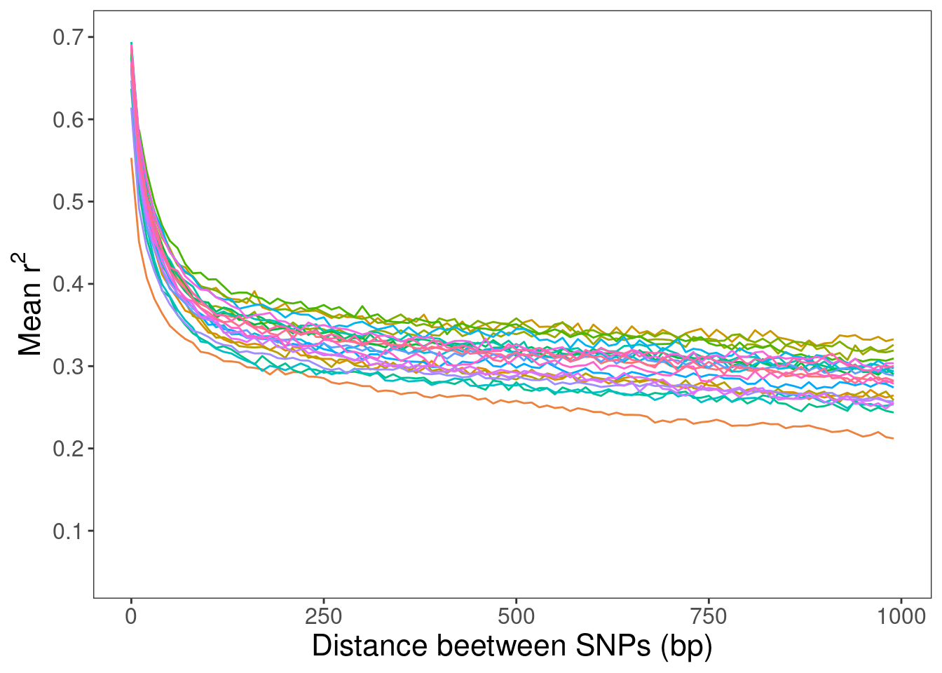
geom_line(aes(bin_bdr, mean, colour = chr)) +
theme_bw() +
xlab("Distance beetween SNPs (bp)") +
ylab(bquote(.("Mean r")^2)) +
labs(colour = "Chromosome") +
theme(panel.grid = element_blank(),
axis.text = element_text(size = 12),
axis.title = element_text(size = 14)) +
guides(colour = F) +
scale_x_continuous(limits = c(0, 1000)) +
scale_y_continuous(breaks = c(0.1, 0.2, 0.3, 0.4, 0.5, 0.6),
limits = c(0.05, 0.6))
## Warning: `guides(<scale> = FALSE)` is deprecated. Please use `guides(<scale> = "none")` instead.
# Save to repo
ggsave(filename = paste("20200803_mean-r2_1kb-lim_MIKK_inset_100bp-bins", ".png", sep = ""),
       plot = r2_1kb_mikk,
       device = "png",
       path = here::here("mikk_genome", "plots"),
       width = 10.88,
       height = 8,
       units = "cm",
       dpi = 500)
10-bp windows
For a finer resolution.
Get means for each bin
script=mikk_genome/code/scripts/20200724_r2_decay_mean_1gk_1kb-lim.R
out_dir=ld/20200727_mean_r2_1kb-lim_mikk

for in_file in $(find ld/20200727_mikk_maf-0.10_window-50kb_no-missing/*ld); do
  name=$(basename $in_file | cut -f1 -d".");
  bsub \
    -M 30000 \
    -o log/20200803_$name\_mean-r2_1kb-max.out \
    -e log/20200803_$name\_mean-r2_1kb-max.err \
    "Rscript \
      --vanilla \
      $script \
      $in_file \
      $out_dir";
done
# Combine in R
data_files <- list.files("ld/20200727_mean_r2_1kb-lim_mikk",
                         full.names = T)

data_files_trunc <- list.files("ld/20200727_mean_r2_1kb-lim_mikk")

data_files_trunc <- gsub(".txt", "", data_files_trunc)

data_list <- lapply(data_files, function(data_file){
  df <- read.delim(data_file,
                   sep = "\t",
                   header = T)
  return(df)
})

names(data_list) <- as.integer(data_files_trunc)

# reorder
data_list <- data_list[order(as.integer(names(data_list)))]

# bind into DF
r2_df_1kb_mikk <- dplyr::bind_rows(data_list, .id = "chr")
r2_df_1kb_mikk$chr <- factor(r2_df_1kb_mikk$chr, levels = seq(1, 24))

# write to table
write.table(r2_df_1kb_mikk, here::here("mikk_genome", "data", "20200803_mikk_ld-decay_1kb-lim_10bp-windows.txt"),
            quote = F, row.names = F, col.names = T, sep = "\t")
Plot
# Read in data
r2_df_1kb_mikk = read.table(here::here("data", "20200803_mikk_ld-decay_1kb-lim_10bp-windows.txt"),
                            header = T, sep = "\t", as.is = T)


# Factorise chromosomes
r2_df_1kb_mikk$chr <- factor(r2_df_1kb_mikk$chr, levels = seq(1, 24))

# Plot
r2_df_1kb_mikk %>% ggplot() +
  geom_line(aes(bin_bdr, mean, colour = chr)) +
  theme_bw() +
  xlab("Distance beetween SNPs (bp)") +
  ylab(bquote(.("Mean r")^2)) +
  labs(colour = "Chromosome") +
  theme(panel.grid = element_blank(),
        axis.text = element_text(size = 12),
        axis.title = element_text(size = 16)) +
  guides(colour = F) +
  scale_y_continuous(breaks = c(0.1, 0.2, 0.3, 0.4, 0.5, 0.6, 0.7),
                     limits = c(0.05, 0.7))
## Warning: `guides(<scale> = FALSE)` is deprecated. Please use `guides(<scale> = "none")` instead.
## Warning: Removed 3 row(s) containing missing values (geom_path).
# Save
ggsave(filename = paste("20200803_mean-r2_1kb-lim_MIKK_inset_10bp-windows", ".png", sep = ""),
       device = "png",
       path = here::here("mikk_genome", "plots"),
       width = 10.88,
       height = 8,
       units = "cm",
       dpi = 500)
MAF distribution MIKK v 1KG
Get frequencies with plink
# 1KG
plink \
  --bfile plink/20200723_1gk_no-missing/20200723 \
  --freq \
  --out maf/20200727_1kg_no-missing
# Creates a 3.9GB file.

# MIKK
plink \
  --bfile plink/20200716_panel_no-sibs_line-ids_no-missing/20200716 \
  --freq \
  --chr-set 24 no-xy \
  --out maf/20200727_mikk_no-missing
# Creates a 657MB file.
Plot
in_mikk <- "../maf/20200727_mikk_no-missing.frq"
in_1kg <- "../maf/20200727_1kg_no-missing.frq"
#out_file <- args[3]

## MIKK
maf_mikk <- readr::read_delim(in_mikk,
                             delim = " ",
                             trim_ws = T,
                             col_types = cols_only(MAF = col_double()))
maf_mikk$dataset <- "MIKK panel"

## 1KG
maf_1kg <- readr::read_delim(in_1kg,
                             delim = " ",
                             trim_ws = T,
                             col_types = cols_only(MAF = col_double()))
maf_1kg$dataset <- "1000 Genomes"

## Bind
maf_final <- rbind(maf_mikk, maf_1kg)

# Plot
maf_plot = maf_final %>%
  ggplot() +
    geom_histogram(aes(x = MAF,
                       y=0.01*..density..,
                       fill = dataset),
                   binwidth = 0.01) +
    theme_cowplot() +
    guides(fill = F) +
    facet_wrap(~dataset, nrow = 1, ncol = 2) +
    xlab("Minor allele frequencies") +
    ylab("Density") +
    theme(strip.background = element_blank(),
          strip.text = element_text(size = 14,
                                    face = "bold"))
LD decay without labels
r2_plot_main_nolabs = r2_final_df %>% ggplot() +
  geom_line(aes(bin_bdr_kb, mean, colour = chr)) +
  theme_cowplot() +
  xlab("Distance between SNPs (kb)") +
  ylab(bquote(.("Mean r")^2)) +
  facet_wrap(~dataset, nrow = 1, ncol = 2) +
  theme(panel.grid = element_blank(),
        strip.background = element_blank(),
        strip.text.x = element_blank(),
        legend.position = c(.9, .8),
        legend.key.size = unit(9, "points"),
        legend.title = element_text(size = 9),
        legend.text = element_text(size = 9)) +
  labs(colour = "Chromosome") +
  scale_y_continuous(breaks = c(0.1, 0.2, 0.3, 0.4, 0.5, 0.6),
                     limits = c(0.05, 0.6))
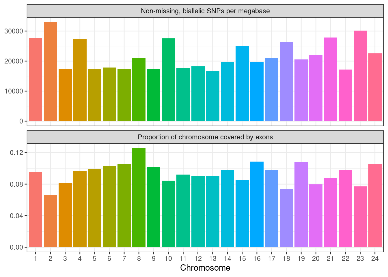
Investigation of LD decay in chr 2
Chromosome 2 has an obviously faster LD decay than the other chromosomes. We explore some possible reasons for this.
Get lengths of each chr on bash
seq 1 24 > tmp1.txt

grep ">" refs/Oryzias_latipes.ASM223467v1.dna.toplevel.fa | scut -f6 -d":" | head -24 > tmp2.txt

paste tmp1.txt tmp2.txt > mikk_genome/data/Oryzias_latipes.ASM223467v1.dna.toplevel.fa_chr_counts.txt
Get proportion of each chromosome covered by exons using biomaRt
# Load libraries
library(here)
source(here::here("code", "scripts", "ld_decay", "source.R"))

# Get length of chromosomes
chr_counts <- readr::read_tsv(here::here("data",
                                         "Oryzias_latipes.ASM223467v1.dna.toplevel.fa_chr_counts.txt"),
                              col_names = c("chr", "length")) %>%
  dplyr::filter(chr != "MT") %>%
  dplyr::mutate(chr = as.integer(chr))

# List marts
listMarts()
##                biomart                version
## 1 ENSEMBL_MART_ENSEMBL      Ensembl Genes 105
## 2   ENSEMBL_MART_MOUSE      Mouse strains 105
## 3     ENSEMBL_MART_SNP  Ensembl Variation 105
## 4 ENSEMBL_MART_FUNCGEN Ensembl Regulation 105
# Select database and list datasets within
ensembl_mart <- useMart("ENSEMBL_MART_ENSEMBL")

# Select dataset
ensembl_olat <- useDataset("olatipes_gene_ensembl", mart = ensembl_mart)
olat_mart = useEnsembl(biomart = "ensembl", dataset = "olatipes_gene_ensembl")
# Get attributes of interest (exon ID, chr, start, end)
exons <- getBM(attributes = c("chromosome_name",
                              "ensembl_gene_id",
                              "ensembl_transcript_id",
                              "transcript_start",
                              "transcript_end",
                              "transcript_length",
                              "ensembl_exon_id",
                              "rank",
                              "strand",
                              "exon_chrom_start",
                              "exon_chrom_end",
                              "cds_start",
                              "cds_end"),
               mart = olat_mart)

# Factorise chr so it's in the right order
chrs <- unique(exons$chromosome_name)
auto_range <- range(as.integer(chrs), na.rm = T)
non_auto <- chrs[is.na(as.integer(chrs))]
chr_order <- c(seq(auto_range[1], auto_range[2]), non_auto)
exons$chromosome_name <- factor(exons$chromosome_name, levels = chr_order)

# Convert into list
exons_lst <- split(exons, f = exons$chromosome_name)

# Get mean length of exons per chromosome
exons_lst <- lapply(exons_lst, function(chr){
  chr <- chr %>%
    dplyr::mutate(exon_length = (exon_chrom_end - exon_chrom_start) + 1,
                  transcript_total_length = (transcript_end - transcript_start) + 1)
  return(chr)
})

# Get total length of chr covered by exons
exon_lengths <- lapply(exons_lst, function(chr){
  # create list of start pos to end pos sequences for each exon
  out_list <- apply(chr, 1, function(exon) {
    seq(exon[["exon_chrom_start"]], exon[["exon_chrom_end"]])
  })
  # combine list of vectors into single vector and get only unique numbers
  out_vec <- unique(unlist(out_list))
  # get length of out_vec and put it into data frame
  out_final <- data.frame("exon_cov" = length(out_vec))
  return(out_final)
})

# combine into single DF
exons_len_df <- dplyr::bind_rows(exon_lengths, .id = "chr") %>%
  dplyr::mutate(chr = as.integer(chr))

# join with chr_counts and get proportion of chr covered by exons
chr_stats <- dplyr::left_join(chr_counts, exons_len_df, by = "chr") %>%
  dplyr::mutate(prop_cov_exon = exon_cov / length)
# convert chr to factor for plotting
chr_stats$chr <- factor(chr_stats$chr)
Get SNP counts per megabase
Get counts
bcftools index \
  --stats \
  ../vcfs/panel_no-sibs_line-ids_no-missing_bi-snps_with-af.vcf.gz \
    > data/20201106_non-missing_bi-snp_count.txt
Read SNP counts data into R
snp_counts = read.table(here::here("data", "20201106_non-missing_bi-snp_count.txt"),
                        sep = "\t",
                        col.names = c("chr", "length", "snp_count")) %>%
  # create megabase column
  dplyr::mutate(megabases = length / 1e6,
                snps_per_megabase = snp_count / megabases) %>%
  # remove MT
  dplyr::filter(chr != "MT") %>%
  # turn chr column into integer
  dplyr::mutate(chr = as.factor(as.integer(chr)))
Combine SNP counts with exon proportion counts
chr_df = snp_counts %>%
  dplyr::full_join(chr_stats, by = c("chr", "length"))

# Create recode vector
recode_vec = c("Non-missing, biallelic SNPs per megabase",
               "Proportion of chromosome covered by exons")
names(recode_vec) = c("snps_per_megabase",
                      "prop_cov_exon")
Plot
chr_df %>%
  tidyr::pivot_longer(cols = c(snps_per_megabase, prop_cov_exon),
                      names_to = "variable",
                      values_to = "values") %>%
  dplyr::mutate(variable = dplyr::recode(variable, !!!recode_vec)) %>%
  ggplot() +
    geom_col(aes(chr, values, fill = chr)) +
    guides(fill = F) +
    xlab("Chromosome") +
    ylab(NULL) +
    theme_bw() +
    facet_wrap(~variable,
               nrow = 2, ncol = 1,
               scales = "free_y")
## Warning: `guides(<scale> = FALSE)` is deprecated. Please use `guides(<scale> = "none")` instead.
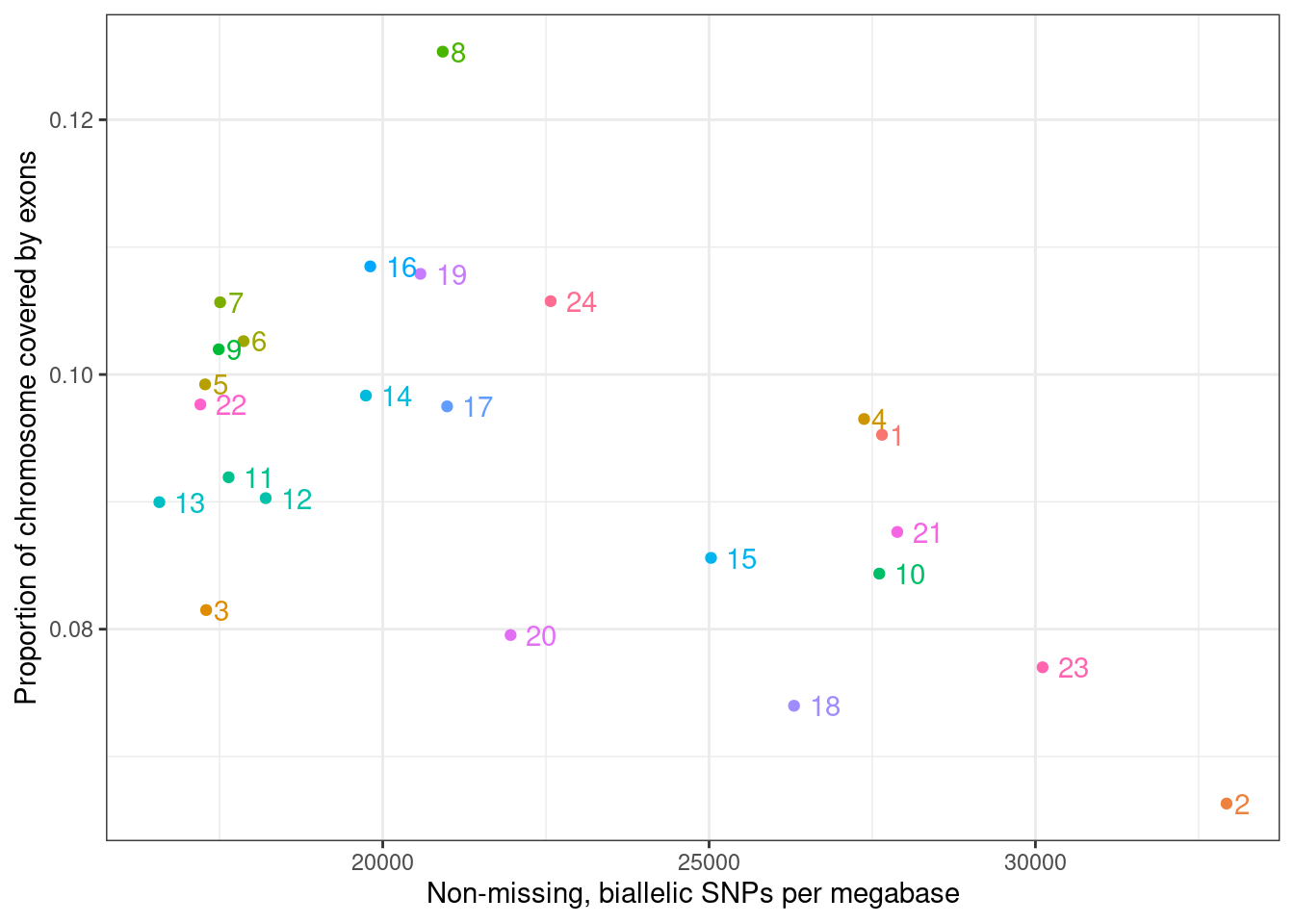
chr_df %>%
  ggplot(aes(snps_per_megabase, prop_cov_exon, colour = chr, label = chr)) +
  geom_point() +
  geom_text(hjust = -0.5) +
  theme_bw() +
  guides(colour = F) +
  xlab("Non-missing, biallelic SNPs per megabase") +
  ylab("Proportion of chromosome covered by exons")
## Warning: `guides(<scale> = FALSE)` is deprecated. Please use `guides(<scale> = "none")` instead.
# Save to repo
ggsave(filename = paste("20201106_snps-per-mb_v_exon-props", ".png", sep = ""),
       device = "png",
       path = here("mikk_genome", "plots"),
       width = 24,
       height = 20,
       units = "cm",
       dpi = 500)
Calculate correlation
cor.test(chr_df$snps_per_megabase, chr_df$prop_cov_exon, method = "spearman")
##
##  Spearman's rank correlation rho
##
## data:  chr_df$snps_per_megabase and chr_df$prop_cov_exon
## S = 3274, p-value = 0.04033
## alternative hypothesis: true rho is not equal to 0
## sample estimates:
##        rho
## -0.4234783
Calculate linkage distance in chr2 relative to other chromosomes
From Naruse et al., Genetics, 2000 (https://www.genetics.org/content/154/4/1773) Table 4:
cms = c(44.2, 85.4, 84.3, 73.5, 66, 82.4, 39, 57.4, 54.3, 71.5, 39.4, 36.6, 48.9, 68.1, 58.1, 57.9, 74.7, 59.8, 47.4, 71.8, 32.3, 29.7, 47.4, 24.4)
names(cms) = 1:24

# cM/Mb
cms_per_mb = cms / (chroms$end / 1e6)
cms_per_mb
<<<<<<< HEAD
##        1        2        3        4        5        6        7        8        9       10       11       12       13       14       15       16
## 1.172005 3.364978 2.203999 2.236159 1.987647 2.555297 1.128035 2.187554 1.625777 2.290307 1.396642 1.198292 1.445643 2.225564 1.906416 1.756745
##       17       18       19       20       21       22       23       24
## 2.349631 1.934099 1.860803 2.767696 1.036958 1.024964 1.942559 1.030304
=======
##        1        2        3        4        5        6        7        8        9       10       11       12       13
## 1.172005 3.364978 2.203999 2.236159 1.987647 2.555297 1.128035 2.187554 1.625777 2.290307 1.396642 1.198292 1.445643
##       14       15       16       17       18       19       20       21       22       23       24
## 2.225564 1.906416 1.756745 2.349631 1.934099 1.860803 2.767696 1.036958 1.024964 1.942559 1.030304
>>>>>>> 1f72b2c38317bbf9e22e15671a199f851eaded2e
# cM/Mb for chr 2
cms_per_mb[[2]]
## [1] 3.364978
# cM/Mb for the rest
mean(cms_per_mb[-2])
## [1] 1.794048
# range for the rest
range(cms_per_mb[-2])
## [1] 1.024964 2.767696