Email from Tom, 18 January:
1. “Polish” SV calls using Illumina data: https://github.com/smehringer/SViper
Please explore the above - get install and tested.
Nanopore VCF files:
- WITH SEQUENCES:
ll /hps/research1/birney/users/adrien/indigene/analyses/indigene_nanopore_DNA/brain_run2/DNA_analysis/results/SV/sniffles_all_OLD/merged.vcf
- WITHOUT SEQUENCES:
/hps/research1/birney/users/adrien/indigene/analyses/indigene_nanopore_DNA/brain_run2/DNA_analysis/results/SV/sniffles_all/merged.vcf
SViper says: >The vcf file must be a structural variant format (tags instead of sequences, e.g. <DEL>). Also the INFO field must include the END tag, giving the end position of the variant, as well as the SVLEN tag in case of insertions.
Then we need to map Illumina ID to the Nanopore VCF and figure out how to run the polishing.
Once done we need to summarise and describe the SV’s a little with some annotations etc - I will make a start with doing this part and we catchup once you have looked at the polishing
2. catchup with Jack on repeats (both MIKK panel and Nanopore assemblies). - create one plot for each paper
3. Fecundity - I will send you the data and a description of what exactly it is later today. - we will need a general description of the data, descriptive stats and a heritability estimate - plus a single plot or table (for MIKK panel paper)
4. Add to txt within the two documents - we can catch-up on this later in the week.
Polish SV calls with Illumina data
Setup
Working directory on EBI cluster: /hps/research1/birney/users/ian/mikk_paper/mikk_genome/sv_analysis GitHub repo: https://github.com/brettellebi/mikk_genome
Source
library(here)
source(here::here("code/scripts/sv_analysis/source.R"))
Nanopore VCF
/hps/research1/birney/users/adrien/analyses/medaka_DNA_promethion/brain_run2/DNA_analysis/results/SV/sniffles_all/merged.vcf
Created with:
# First used:
sniffles \
  --min_support 3 \
  --max_num_splits 7 \
  --max_distance 1000 \
  --min_length 50 \
  --minmapping_qual 20 \
  --min_seq_size 1000 \
  --allelefreq 0.1 \
  -t {threads} \
  -m {input_bam} \
  -v {output_vcf}
Adrien: >Then I filtered and merged all the variants from the different samples together with survivor and recalled variants a second time in forced mode using the merged set with sniffles again using the same options.
Copy to working directory
# With sequences
nano_raw=/hps/research1/birney/users/adrien/indigene/analyses/indigene_nanopore_DNA/brain_run2/DNA_analysis/results/SV/sniffles_all_OLD/merged.vcf
out_path=../sv_analysis/vcfs/ont_raw_with_seq.vcf
## Copy
cp $nano_raw $out_path

# Without sequences
nano_raw=/hps/research1/birney/users/adrien/indigene/analyses/indigene_nanopore_DNA/brain_run2/DNA_analysis/results/SV/sniffles_all/merged.vcf
out_path=../sv_analysis/vcfs/ont_raw.vcf
## Copy
cp $nano_raw $out_path
Rename samples
With sequences
conda activate sv_env

in_vcf=../sv_analysis/vcfs/ont_raw_with_seq.vcf
sample_file=data/sv_analysis/20210205_ont_raw_samples_file.txt
out_vcf=../sv_analysis/vcfs/ont_raw_with_seq_rehead.vcf

# Make samples key file
bcftools query -l $in_vcf \
  > tmp1
cut -f4 -d'/' tmp1 | cut -f1 -d'_' \
  > tmp2
paste -d' ' tmp1 tmp2 > $sample_file
rm tmp1 tmp2

# Rename VCF
bcftools reheader \
  --samples $sample_file \
  --output $out_vcf \
  $in_vcf
Without sequences
conda activate sv_env

in_vcf=../sv_analysis/vcfs/ont_raw.vcf
sample_file=data/sv_analysis/20210212_ont_raw_samples_file.txt
out_vcf=../sv_analysis/vcfs/ont_raw_rehead.vcf

# Make samples key file
bcftools query -l $in_vcf \
  > tmp1
cut -f4 -d'/' tmp1 | cut -f1 -d'_' \
  > tmp2
paste -d' ' tmp1 tmp2 > $sample_file
rm tmp1 tmp2

# Rename VCF
bcftools reheader \
  --samples $sample_file \
  --output $out_vcf \
  $in_vcf
Get stats
With sequences
conda activate sv_mikk

in_vcf=../sv_analysis/vcfs/ont_raw_with_seq.vcf
stats_out=../sv_analysis/vcfs/ont_raw_with_seq.stats

# Get stats
bcftools stats \
  $in_vcf \
    > $stats_out
Without sequences
conda activate sv_mikk

in_vcf=../sv_analysis/vcfs/ont_raw.vcf
stats_out=../sv_analysis/vcfs/ont_raw.stats

# Get stats
bcftools stats \
  $in_vcf \
    > $stats_out
Split per sample
With sequences
conda activate sv_mikk

in_vcf=../sv_analysis/vcfs/ont_raw_with_seq_rehead.vcf
out_dir=../sv_analysis/vcfs/ont_raw_with_seq_rehead_per_sample

mkdir -p $out_dir

# Split by sample
bcftools +split \
  $in_vcf \
  --output $out_dir
Without sequences
conda activate sv_mikk

in_vcf=../sv_analysis/vcfs/ont_raw_rehead.vcf
out_dir=../sv_analysis/vcfs/ont_raw_rehead_per_sample

mkdir -p $out_dir

# Split by sample
bcftools +split \
  $in_vcf \
  --output $out_dir
Illumina VCF
Copy to working directory
conda activate sv_env

in_vcf=/nfs/research1/birney/projects/medaka/inbred_panel/medaka-alignments-release-94/vcf/medaka_inbred_panel_ensembl_new_reference_release_94.vcf
out_vcf=../sv_analysis/vcfs/ill_raw.vcf.gz

# Compress and copy
bsub \
  -M 30000 \
  -o ../log/20210208_comp_ill.out \
  -e ../log/20210208_comp_ill.err \
bsub -Is bash \
  """
  conda activate sv_env ;
  bcftools view \
    --output-type z \
    --output $out_vcf \
    $in_vcf
  """
Rename and filter for ONT samples
Pull out IDs for relevant samples
ont_samples = here::here("data", "sv_analysis", "20210205_ont_raw_samples_file.txt")
ill_samples = here::here("data","20200206_cram_id_to_line_id.txt")
out_file = here::here("data", "sv_analysis", "20210205_ill_key_ont_samples.txt")
out_samples = here::here("data", "sv_analysis", "20210205_ont_samples_only.txt")

# Read in tables

ont_key = read.table(ont_samples)
ill_key = read.table(ill_samples, comment.char = "\"", header = T) %>%
  dplyr::mutate(line = gsub("_", "-", line))

# Find matches
out = ill_key[ill_key$line %in% ont_key$V2, ]

# Write to files
## Key file
readr::write_delim(out, out_file, delim = " ", col_names = F)
## Just samples
readr::write_lines(out$cram_file, out_samples)
Rename and filter
in_vcf=../sv_analysis/vcfs/ill_raw.vcf.gz
samples_file=data/sv_analysis/20210205_ont_samples_only.txt
samples_key=data/sv_analysis/20210205_ill_key_ont_samples.txt
out_vcf=../sv_analysis/vcfs/ill_raw_rehead.vcf.gz
out_dir=../sv_analysis/vcfs/ill_raw_rehead_per_sample

mkdir -p $out_dir

# Filter for target samples and rehead
bcftools view \
  --samples-file $samples_file \
  --output-type u \
  $in_vcf |\
    bcftools reheader \
      --samples $samples_key \
      --output $out_vcf

# Split by sample
bcftools +split \
  $out_vcf \
  --output $out_dir
BAMs
Illumina .bam files
Copy to local.
sample_key=data/sv_analysis/20210205_ill_key_ont_samples.txt
ill_bam_dir=/nfs/research1/birney/projects/medaka/inbred_panel/medaka-alignments-release-94/bam
out_dir=../sv_analysis/bams

mkdir -p $out_dir

# Copy over
for sample in $(cut -f1 -d' ' $sample_key ) ; do
  cp $ill_bam_dir/$sample.bai $out_dir ;
done

# SViper needs bams in .bam.bai format. Original {sample}.bai files need to be copied to {sample}.bam.bai
for file in $( find $out_dir/*.bai ) ; do
  new_filename=$( echo $file | sed 's/.bai/.bam.bai/g' ) ;
  mv $file $new_filename ;
done
Nanopore .bam files
Sit here: /hps/research1/birney/users/adrien/indigene/analyses/indigene_nanopore_DNA/brain_run2/DNA_analysis/results/SV/ngmlr_alignments/
Polish Nanopore reads with SViper
Create Singularity container
module load singularity

# Build
singularity build \
  --remote ../sing_conts/sviper.sif \
  envs/sviper/20210204_sviper.def

# Open interactive shell
bsub -Is "singularity shell ../sing_conts/sviper.sif"
# Works!
Test
# Load singularity
module load singularity
# Pull image built with `envs/sviper/20210204_sviper.def`
bsub -M 30000 -n 4 -Is "singularity shell ../sing_conts/sviper.sif"

#######################
# Variables
#######################
## Container
container=../sing_conts/sviper.sif
## Sample
sample=11-1
sample_key=data/sv_analysis/20210205_ill_key_ont_samples.txt
## VCF to polish
ont_vcf=../sv_analysis/vcfs/ont_raw_rehead_per_sample/$sample.vcf
## Illumina BAM
ill_cram_id=$(grep $sample $sample_key | cut -f1 -d' ')
ill_bam_dir=../sv_analysis/bams
ill_bam=$ill_bam_dir/$ill_cram_id.bam
## Nanopore BAM
ont_bam_dir=/hps/research1/birney/users/adrien/indigene/analyses/indigene_nanopore_DNA/brain_run2/DNA_analysis/results/SV/ngmlr_alignments
ont_bam=$(find $ont_bam_dir/$sample*.bam)
## Reference
ref=../refs/Oryzias_latipes.ASM223467v1.dna.toplevel.fa
## Output directory
out_dir=../sv_analysis/vcfs/sviper
mkdir -p $out_dir

#######################
# TEST call sviper
#######################
sviper \
  --candidate-vcf $ont_vcf \
  --short-read-bam $ill_bam \
  --long-read-bam $ont_bam \
  --reference $ref \
  --output-prefix $out_dir/$sample
True
# Load singularity
module load singularity
# Pull image built with `envs/sviper/20210204_sviper.def`
bsub -M 30000 -n 4 -Is "singularity shell ../sing_conts/sviper.sif"

#######################
# Variables
#######################
## Sample
sample=11-1
sample_key=data/sv_analysis/20210205_ill_key_ont_samples.txt
## VCF to polish
ont_vcf=../sv_analysis/vcfs/ont_raw_rehead_per_sample/$sample.vcf
## Illumina BAM
ill_cram_id=$(grep $sample $sample_key | cut -f1 -d' ')
ill_bam_dir=../sv_analysis/bams
ill_bam=$ill_bam_dir/$ill_cram_id.bam
## Nanopore BAM
ont_bam_dir=/hps/research1/birney/users/adrien/indigene/analyses/indigene_nanopore_DNA/brain_run2/DNA_analysis/results/SV/ngmlr_alignments
ont_bam=$(find $ont_bam_dir/$sample*.bam)
## Reference
ref=../refs/Oryzias_latipes.ASM223467v1.dna.toplevel.fa
## Container
container=../sing_conts/sviper.sif
## Output directory
out_dir=../sv_analysis/vcfs/sviper
mkdir -p $out_dir

#######################
# TEST call sviper
#######################
sviper \
  --candidate-vcf $ont_vcf \
  --short-read-bam $ill_bam \
  --long-read-bam $ont_bam \
  --reference $ref \
  --output-prefix $out_dir/$sample

#######################
# TRUE call sviper
#######################
module load singularity

# Global variables
## Sample key
sample_key=data/sv_analysis/20210205_ill_key_ont_samples.txt
## BAM dirs
ill_bam_dir=../sv_analysis/bams
ont_bam_dir=/hps/research1/birney/users/adrien/indigene/analyses/indigene_nanopore_DNA/brain_run2/DNA_analysis/results/SV/ngmlr_alignments
## Reference
ref=../refs/Oryzias_latipes.ASM223467v1.dna.toplevel.fa
## Container
container=../sing_conts/sviper.sif
## Output directory
out_dir=../sv_analysis/vcfs/sviper
mkdir -p $out_dir

for sample in $(cut -f2 -d' ' $sample_key | tail -n+2 ) ; do
  # Set variables

  ## VCF to polish
  ont_vcf=../sv_analysis/vcfs/ont_raw_rehead_per_sample/$sample.vcf
  ## Illumina BAM
  ill_cram_id=$(grep " $sample" $sample_key | cut -f1 -d' ')
  ill_bam=$ill_bam_dir/$ill_cram_id.bam
  ## Nanopore BAM
  ont_bam=$(find $ont_bam_dir/$sample*.bam)

  # Run SViper
  bsub \
    -M 30000 \
    -n 16 \
    -o ../log/20210212_sviper_$sample.out \
    -e ../log/20210212_sviper_$sample.err \
    """
    singularity exec $container \
      sviper \
        --candidate-vcf $ont_vcf \
        --short-read-bam $ill_bam \
        --long-read-bam $ont_bam \
        --reference $ref \
        --output-prefix $out_dir/$sample
    """
done

# 4-2 and 7-2 failed with no error message
Merge
# Get list of vcf paths
in_dir=../sv_analysis/vcfs/sviper
out_dir=$in_dir/merged
mkdir -p $out_dir
in_vcfs=$(find $in_dir/*.vcf | tr '\n' ' ')

bcftools merge \
  --output $out_dir/all.vcf\
  $in_vcfs

# Requires them to be bgzipped

# Try with Picard
in_dir=../sv_analysis/vcfs/sviper
out_dir=$in_dir/merged
mkdir -p $out_dir
find $in_dir/*.vcf > tmp.list

picard MergeVcfs \
  I=tmp.list \
  O=$out_dir/merged.vcf.gz

rm tmp.list
#Exception in thread "main" java.lang.IllegalArgumentException: Input file /hps/research1/birney/users/ian/mikk_paper/mikk_genome/../sv_analysis/vcfs/sviper/117-2.vcf has sample entries that don't match the other files.
Get data from SViper
in_dir=../sv_analysis/vcfs/sviper
out_dir=data/sv_analysis/20210217_sviper_filter_pass

mkdir -p $out_dir

for in_vcf in $(find $in_dir/*vcf) ; do
  sample=$(basename $in_vcf | cut -f1 -d'.' ) ;
  bcftools query \
    --exclude 'GT~"\."' \
    --format '%CHROM,%POS,%ID,%ALT,%FILTER,%INFO/SVLEN,%INFO/SVTYPE,%INFO/CHR2,%INFO/END,[%GT],[%LN],[%ST]\n' \
  --output $out_dir/$sample.csv \
  $in_vcf ;
done
Get data from original VCF
in_dir=../sv_analysis/vcfs/ont_raw_rehead_per_sample
out_dir=data/sv_analysis/20210217_raw_ont_filter_pass

mkdir -p $out_dir

for in_vcf in $(find $in_dir/*vcf) ; do
  sample=$(basename $in_vcf | cut -f1 -d'.' ) ;
  bcftools query \
    --include 'FILTER="PASS"' \
    --exclude 'GT~"\."' \
    --format '%CHROM,%POS,%ID,%ALT,%FILTER,%INFO/SVLEN,%INFO/SVTYPE,%INFO/CHR2,%INFO/END,[%GT],[%LN],[%ST]\n' \
  --output $out_dir/$sample.csv \
  $in_vcf ;
done
Analysis
Read in SV data
SViper polished
in_dir = here::here("data", "sv_analysis/20210217_sviper_filter_pass")

in_files = list.files(in_dir, full.names = T)
names(in_files) = basename(in_files) %>%
  str_remove(".csv")

sv_df_pol = lapply(in_files, function(in_file){
  df = readr::read_csv(in_file,
                       col_names = c("CHROM", "POS", "ID", "ALT", "FILTER", "SVLEN", "SVTYPE", "CHR2", "END", "GT", "LN", "ST"),
                       col_types = c("ciicciccicic"))

  return(df)
}) %>%
  dplyr::bind_rows(.id = "SAMPLE") %>%
  # add "chr" to beginning of CHROM column
  dplyr::mutate(CHROM = paste("chr", CHROM, sep = ""))
Counts for FILTER by SVTYPE
sv_df_pol %>%
  # Remove 131-1
  dplyr::filter(SAMPLE %in% ont_samples_pol) %>%
  dplyr::group_by(SVTYPE, FILTER) %>%
  dplyr::count()
## # A tibble: 14 × 3
## # Groups:   SVTYPE, FILTER [14]
##    SVTYPE FILTER      n
##    <chr>  <chr>   <int>
##  1 DEL    FAIL1     182
##  2 DEL    FAIL2   16638
##  3 DEL    FAIL4      49
##  4 DEL    FAIL5    9720
##  5 DEL    PASS   333373
##  6 DUP    SKIP    23991
##  7 INS    FAIL1     430
##  8 INS    FAIL2   30286
##  9 INS    FAIL4      71
## 10 INS    FAIL5    8297
## 11 INS    PASS   265857
## 12 INS    SKIP        2
## 13 INV    SKIP     5549
## 14 TRA    SKIP    31382
**SViper only polishes insertions and deletions! Actually says that in the first line of the README. Will have to conditionally filter.
How many DUP and INS filtered out?
sv_df_pol %>%
  dplyr::filter(SAMPLE %in% ont_samples_pol) %>%
  dplyr::filter(SVTYPE %in% c("DEL", "INS")) %>%
  dplyr::group_by(SVTYPE, FILTER) %>%
  dplyr::count() %>%
  dplyr::ungroup() %>%
  split(., f = .$SVTYPE) %>%
  purrr::map(function(x) {
    data.frame(TOTAL = sum(x$n),
               TOTAL_FAILED = sum(x %>%
                                    dplyr::filter(FILTER != "PASS") %>%
                                    dplyr::select(n)),
               TOTAL_PASSED = x %>%
                 dplyr::filter(FILTER == "PASS") %>%
                 dplyr::pull(n)) %>%
      dplyr::mutate(PROP_FAILED = TOTAL_FAILED / TOTAL)
    }) %>%
  dplyr::bind_rows(.id = "SVTYPE")
##   SVTYPE  TOTAL TOTAL_FAILED TOTAL_PASSED PROP_FAILED
## 1    DEL 359962        26589       333373  0.07386613
## 2    INS 304943        39086       265857  0.12817477
Plot frequency of different types of fails
sv_filter_desc = sv_df_pol %>%
  # remove 131-1
  dplyr::filter(SAMPLE %in% ont_samples_pol) %>%
  dplyr::group_by(SVTYPE, FILTER) %>%
  dplyr::mutate(FILTER = factor(FILTER, levels = names(filter_recode)),
                FILTER_DESC = dplyr::recode(FILTER, !!!filter_recode)) %>%
  dplyr::filter(SVTYPE %in% c("DEL", "INS")) %>%
  ggplot() +
    geom_bar(aes(FILTER_DESC, fill = SVTYPE)) +
    theme_bw() +
    theme(axis.text.x = element_text(size = 5)) +
    facet_wrap(~SVTYPE) +
    scale_fill_manual(values = svtype_hist_pal) +
    xlab("Filter description") +
    guides(fill = "none")
ggsave(here::here("docs/plots/sv_analysis/20210325_sv_filter.png"),
       device = "png",
       width = 20,
       height = 9.375,
       units = "cm",
       dpi = 400)
<<<<<<< HEAD
=======
>>>>>>> 1f72b2c38317bbf9e22e15671a199f851eaded2e
# Make copy of full polished DF
sv_df_pol_all = sv_df_pol

# Filter out non-passes for DEL and INS STYPEs
sv_df_pol = sv_df_pol %>%
  dplyr::filter(SAMPLE %in% ont_samples_pol) %>%
  dplyr::filter(!(SVTYPE %in% c("DEL", "INS") & FILTER != "PASS"))


sv_df_pol %>%
  dplyr::group_by(SVTYPE, FILTER) %>%
  dplyr::count()
## # A tibble: 5 × 3
## # Groups:   SVTYPE, FILTER [5]
##   SVTYPE FILTER      n
##   <chr>  <chr>   <int>
## 1 DEL    PASS   333373
## 2 DUP    SKIP    23991
## 3 INS    PASS   265857
## 4 INV    SKIP     5549
## 5 TRA    SKIP    31382
ONT unpolished
in_dir = here::here("data", "sv_analysis/20210217_raw_ont_filter_pass")

in_files = list.files(in_dir, full.names = T)
names(in_files) = basename(in_files) %>%
  str_remove(".csv")

sv_df_raw = lapply(in_files, function(in_file){
  df = readr::read_csv(in_file,
                       col_names = c("CHROM", "POS", "ID", "ALT", "FILTER", "SVLEN", "SVTYPE", "CHR2", "END", "GT", "LN", "ST"),
                       col_types = c("ciicciccicic"))

  return(df)
}) %>%
  dplyr::bind_rows(.id = "SAMPLE") %>%
  # add "chr" to beginning of CHROM column
  dplyr::mutate(CHROM = paste("chr", CHROM, sep = ""))
Combine into single df
# All
sv_df_all = list("polished" = sv_df_pol_all,
             "unpolished" = sv_df_raw) %>%
  dplyr::bind_rows(.id = "DATASET") %>%
  # factor samples and dataset
  dplyr::mutate(SAMPLE = factor(SAMPLE, levels = ont_samples),
                DATASET = factor(DATASET, levels = c("unpolished", "polished")))

# Filtered
sv_df = list("polished" = sv_df_pol,
             "unpolished" = sv_df_raw) %>%
  dplyr::bind_rows(.id = "DATASET") %>%
  # factor samples and dataset
  dplyr::mutate(SAMPLE = factor(SAMPLE, levels = ont_samples),
                DATASET = factor(DATASET, levels = c("unpolished", "polished")))
How many SVs did polishing change?
NOTE: there is a small number of SV IDs that are duplicated, e.g.:
sv_df_all %>% dplyr::filter(SAMPLE == "4-1" & ID == 78181)
## # A tibble: 4 × 14
##   DATASET    SAMPLE CHROM      POS    ID ALT   FILTER SVLEN SVTYPE CHR2       END GT       LN ST
##   <fct>      <fct>  <chr>    <int> <int> <chr> <chr>  <int> <chr>  <chr>    <int> <chr> <int> <chr>
## 1 polished   4-1    chr9  29694756 78181 <INS> PASS    1215 INS    9     29694755 0/1    1215 +-
## 2 polished   4-1    chr9  29694756 78181 <INS> PASS    1218 INS    9     29694755 0/0    1218 +-
## 3 unpolished 4-1    chr9  29694756 78181 <INS> PASS    1215 INS    9     29694755 0/1    1215 +-
## 4 unpolished 4-1    chr9  29694756 78181 <INS> PASS    1218 INS    9     29694755 0/0    1218 +-
# How many duplicates?
sv_df_all %>%
  dplyr::filter(SVTYPE %in% c("DEL", "INS") & FILTER == "PASS") %>%
  group_by(DATASET, SAMPLE) %>%
  summarise(length(which(duplicated(ID))))
## `summarise()` has grouped output by 'DATASET'. You can override using the `.groups` argument.
## # A tibble: 22 × 3
## # Groups:   DATASET [2]
##    DATASET    SAMPLE `length(which(duplicated(ID)))`
##    <fct>      <fct>                            <int>
##  1 unpolished 4-1                                  5
##  2 unpolished 4-2                                  3
##  3 unpolished 7-1                                  1
##  4 unpolished 7-2                                  3
##  5 unpolished 11-1                                 0
##  6 unpolished 69-1                                 1
##  7 unpolished 79-2                                 2
##  8 unpolished 80-1                                 0
##  9 unpolished 117-2                                0
## 10 unpolished 131-1                                4
## # … with 12 more rows
Exclude duplicates and get percentages of amended POS, END, and LN
polish_comp_list = sv_df_all %>%
  # Refactorise to exclude unpolished ONT samples
  dplyr::mutate(SAMPLE = factor(SAMPLE, levels = ont_samples_pol)) %>%
  # Take only polished samples
  dplyr::filter(SAMPLE %in% ont_samples_pol) %>%
  # Take only DEL and INS that passed the filter
  dplyr::filter(SVTYPE %in% c("DEL", "INS") & FILTER == "PASS") %>%
  # Remove duplicates
  dplyr::group_by(DATASET, SAMPLE) %>%
  dplyr::filter(!duplicated(ID)) %>%
  dplyr::ungroup() %>%
  # Take target columns
  dplyr::select(DATASET, SAMPLE, ID, CHROM, POS, END, LN) %>%
  # Split by sample and run following on each
  split(., .$SAMPLE) %>%
  purrr::map(., function(sample) sample %>%
    # Pivot wider by DATASET to compare POS, END and LN
    tidyr::pivot_wider(id_cols = c(DATASET, ID),
                       names_from = DATASET,
                       values_from = c(POS, END, LN),
                       ) %>%
    # Get proportions of SVs where unpolished and polished differ in POS, END, or LN
    dplyr::mutate(POS_diff = abs(POS_polished - POS_unpolished),
                  END_diff = abs(END_polished - END_unpolished),
                  LN_diff = abs(LN_polished - LN_unpolished)) #%>%
#    dplyr::summarise(TOTAL = n(),
#                     dplyr::across(ends_with("_diff"), ~sum(.x > 0, na.rm = T)/TOTAL))
  ) #%>%
  #dplyr::bind_rows(.id = "SAMPLE")

polish_comp_list %>%
  purrr::map(., function(sample) sample %>%
    dplyr::summarise(TOTAL = n(),
                     dplyr::across(tidyselect::ends_with("_diff"),
                                   ~sum(.x, na.rm = T)/TOTAL))
  ) %>%
  dplyr::bind_rows(.id = "SAMPLE")
## # A tibble: 9 × 5
##   SAMPLE TOTAL POS_diff END_diff  LN_diff
##   <chr>  <int>    <dbl>    <dbl>    <dbl>
## 1 4-1    73686     21.7     27.4 0.00919
## 2 7-1    72936     20.3     26.5 0
## 3 11-1   74354     20.9     26.2 0
## 4 69-1   71377     21.5     29.3 0
## 5 79-2   72983     20.8     27.1 0.00134
## 6 80-1   75129     18.5     24.1 0
## 7 117-2  74284     20.4     29.0 0
## 8 134-1  75632     20.6     29.7 0.000423
## 9 134-2  74508     21.7     26.1 0
Average difference in breakpoints
# Per sample
polish_comp_list %>%
  purrr::map(., function(sample) sample %>%
    dplyr::summarise(TOTAL = n(),
                     dplyr::across(ends_with("_diff"), ~mean(.x, na.rm = T)))
  ) %>%
  dplyr::bind_rows(.id = "SAMPLE")
## # A tibble: 9 × 5
##   SAMPLE TOTAL POS_diff END_diff  LN_diff
##   <chr>  <int>    <dbl>    <dbl>    <dbl>
## 1 4-1    73686     24.0     30.4 0.0102
## 2 7-1    72936     22.5     29.4 0
## 3 11-1   74354     23.2     29.1 0
## 4 69-1   71377     23.9     32.6 0
## 5 79-2   72983     23.0     30.1 0.00149
## 6 80-1   75129     20.7     26.9 0
## 7 117-2  74284     22.6     32.2 0
## 8 134-1  75632     22.8     32.9 0.000469
## 9 134-2  74508     24.0     28.9 0
# Mean of means
polish_comp_list %>%
  purrr::map(., function(sample) sample %>%
    dplyr::summarise(TOTAL = n(),
                     dplyr::across(ends_with("_diff"), ~mean(.x, na.rm = T)))
  ) %>%
  dplyr::bind_rows(.id = "SAMPLE") %>%
  dplyr::summarise(dplyr::across(ends_with("_diff"), ~mean(.x)))
## # A tibble: 1 × 3
##   POS_diff END_diff LN_diff
##      <dbl>    <dbl>   <dbl>
## 1     23.0     30.3 0.00135
Plot counts of polished SV types
# Histogram of LN
svtype_distinct_df = sv_df %>%
  # Extract polished data and remove TRA
  dplyr::filter(DATASET == "polished",
                SVTYPE != "TRA") %>%
  # Remove polish-filter fails
  dplyr::filter(!(SVTYPE %in% c("DEL", "INS") & FILTER != "PASS")) %>%
  dplyr::mutate(SVTYPE = factor(SVTYPE, levels = c("DEL", "INS", "DUP", "INV"))) %>%
  dplyr::select(SVTYPE, CHROM, POS, END, LN) %>%
  dplyr::distinct()

svlen_counts_plot = svtype_distinct_df %>%
  ggplot(aes(x = log10(LN),
             y = ifelse(log10(..count..) < 0,
                        0,
                        log10(..count..)),
             fill = SVTYPE,
             colour = SVTYPE)) +
    geom_area(stat = "bin",
              bins = 100) +
    scale_fill_manual(values = svtype_hist_pal) +
    scale_colour_manual(values = karyoploteR::darker(svtype_hist_pal)) +
    guides(fill = "none") +
    guides(colour = "none") +
    scale_x_continuous(breaks = seq(1, 6, 1),
                       limits = c(1, 6)) +
    facet_wrap(~SVTYPE, nrow = 2, ncol = 2) +
    xlab(expression(log[10](length))) +
    ylab(expression(log[10](count))) +
    theme_cowplot() +
    theme(axis.text.x = element_text(size = 6),
          strip.text = element_text(face = "bold"),
          strip.background = element_blank()
          )

svlen_counts_plot

Compare counts of DEL and INS before and after polishing
# Histogram of LN
polish_comp_plot = sv_df %>%
  # take only the samples in the polished dataset
  dplyr::filter(SAMPLE %in% ont_samples_pol) %>%
  dplyr::filter(SVTYPE %in% c("DEL", "INS")) %>%
  # order by SVTYPE
  dplyr::mutate(SVTYPE = factor(SVTYPE, levels = c("DEL", "INS", "DUP", "INV"))) %>%
  dplyr::select(DATASET, CHROM, POS, END, SVTYPE, LN) %>%
  dplyr::distinct() %>%
  ggplot(aes(x = log10(LN),
             y = ifelse(log10(..count..) < 0,
                        0,
                        log10(..count..)),
             fill = SVTYPE,
             colour = SVTYPE)) +
    geom_area(stat = "bin",
              bins = 100) +
    scale_fill_manual(values = svtype_hist_pal) +
    scale_colour_manual(values = karyoploteR::darker(svtype_hist_pal)) +
    guides(fill = "none") +
    guides(colour = "none") +
    scale_x_continuous(breaks = seq(1, 6, 1),
                       limits = c(1, 6)) +
    facet_grid(rows = vars(DATASET),
               cols = vars(SVTYPE)) +
    xlab(expression(log[10](length))) +
    ylab(expression(log[10](count))) +
    theme_cowplot() +
    theme(axis.text.x = element_text(size = 6),
          strip.text = element_text(face = "bold"),
          strip.background = element_blank()
          )

polish_comp_plot

ggsave(here::here("docs/plots/sv_analysis/20210325_polish_count_comparison.png"),
       polish_comp_plot,
       device = "png",
       width = 15,
       height = 9.375,
       units = "cm",
       dpi = 400)
Plot counts of SV types (per sample)
Get order of SV type by frequency
# Get order
type_order = dplyr::count(sv_df, SVTYPE) %>%
  dplyr::arrange(desc(n)) %>%
  dplyr::pull(SVTYPE)

# Set palette
pal_svtype = grDevices::colorRampPalette(pal_brainbow)(length(ont_samples_pol))
names(pal_svtype) = ont_samples_pol
All
sv_counts_all = sv_df %>%
  dplyr::filter(DATASET == "polished") %>%
  group_by(SAMPLE, SVTYPE) %>%
  summarise(N = n()) %>%
  dplyr::mutate(FACET = "TOTAL") %>%
  dplyr::ungroup()
## `summarise()` has grouped output by 'SAMPLE'. You can override using the `.groups` argument.
Singletons
# Create DF with SAMPLE for binding later
sv_df_pol_samps = sv_df %>%
  # exclude raw data, take only polished
  dplyr::filter(DATASET == "polished") %>%
  # select only target cols
  dplyr::select(CHROM, POS, SVTYPE, LN, SAMPLE)

# Create DF without SAMPLE for detecting duplicates
sv_df_pol_dupes = sv_df %>%
  # exclude raw data, take only polished
  dplyr::filter(DATASET == "polished") %>%
  # select only target cols
  dplyr::select(CHROM, POS, SVTYPE, LN)

## Get unique rows
uq_svs = sv_df_pol_dupes[!(duplicated(sv_df_pol_dupes) | duplicated(sv_df_pol_dupes, fromLast = T)), ]

# Join back with other variables
sv_sings = dplyr::right_join(sv_df_pol_samps, uq_svs)
## Joining, by = c("CHROM", "POS", "SVTYPE", "LN")
DT::datatable(head(sv_sings, 100))
<<<<<<< HEAD
=======
>>>>>>> 1f72b2c38317bbf9e22e15671a199f851eaded2e
# Get singleton counts
sv_counts_sings = sv_sings %>%
  dplyr::group_by(SAMPLE, SVTYPE) %>%
  dplyr::summarise(N = n()) %>%
  dplyr::mutate(FACET = "SINGLETONS") %>%
  dplyr::ungroup()
## `summarise()` has grouped output by 'SAMPLE'. You can override using the `.groups` argument.
Bind together and plot
# Bind DFs
sv_counts = dplyr::bind_rows(sv_counts_all,
                             sv_counts_sings) %>%
  dplyr::mutate(FACET = factor(FACET, levels = c("TOTAL", "SINGLETONS")),
                SVTYPE = factor(SVTYPE, levels = type_order))

# Set palette
pal_svcounts = grDevices::colorRampPalette(pal_smrarvo)(length(ont_samples))
names(pal_svcounts) = ont_samples

# Plot
svtype_counts_plot = sv_counts %>%
  ggplot() +
    geom_col(aes(SAMPLE, N, fill = SAMPLE)) +
    facet_grid(rows = vars(FACET),
               cols = vars(SVTYPE),scales = "free_y") +
    scale_fill_manual(values = pal_svcounts) +
    theme_cowplot() +
    theme(strip.background = element_blank(),
          axis.text.x = element_text(size = 5,angle = 45,hjust = 1),
          strip.text.x = element_text(face = "bold")) +
    guides(fill = "none") +
    xlab("Sample") +
    ylab("Count")
ggplotly(svtype_counts_plot)
<<<<<<< HEAD
=======
>>>>>>> 1f72b2c38317bbf9e22e15671a199f851eaded2e
Get summary counts and percentages of SV types
# Min, max and mean counts across samples per SVTYPE
sv_counts %>%
  filter(FACET == "TOTAL") %>%
  # split by SVTYPE
  split(f = .$SVTYPE) %>%
  # get max and min counts across all samples
  map(., function(x){
    data.frame(MIN = min(x$N),
               MAX = max(x$N),
               MEAN = mean(x$N),
               SD = sd(x$N))
  }) %>%
  bind_rows(.id = "SVTYPE")
##   SVTYPE   MIN   MAX       MEAN        SD
## 1    DEL 35852 37841 37041.4444 603.07506
## 2    INS 28295 30464 29539.6667 625.69421
## 3    TRA  3311  3713  3486.8889 137.27932
## 4    DUP  2583  2777  2665.6667  69.93390
## 5    INV   590   634   616.5556  14.62114
# Percentage singletons
sv_counts %>%
  pivot_wider(id_cols = c(SAMPLE, SVTYPE),
              names_from = FACET,
              values_from = N) %>%
  mutate(PERC_SING = SINGLETONS/TOTAL * 100) %>%
  group_by(SVTYPE) %>%
  summarise(max(PERC_SING),
            min(PERC_SING),
            mean(PERC_SING))
## # A tibble: 5 × 4
##   SVTYPE `max(PERC_SING)` `min(PERC_SING)` `mean(PERC_SING)`
##   <fct>             <dbl>            <dbl>             <dbl>
## 1 DEL               12.7             10.8              11.9
## 2 INS               15.4             12.6              14.2
## 3 TRA               10.5              7.06              8.55
## 4 DUP                8.46             6.08              7.09
## 5 INV                9.36             4.33              6.78
# Ranges, mean, and 90th percentiles of SVLEN per SVTYPE
svtype_distinct_df %>%
  group_by(SVTYPE) %>%
  summarise(max(LN),
            min(LN),
            mean(LN),
            quantile(LN, 0.9))
## # A tibble: 4 × 5
##   SVTYPE `max(LN)` `min(LN)` `mean(LN)` `quantile(LN, 0.9)`
##   <fct>      <int>     <int>      <dbl>               <dbl>
## 1 DEL       493854        51      2583.               3815
## 2 INS        13649        51       776.               2053
## 3 DUP       494748        52     19197.              47864.
## 4 INV       499229        53     70524.             290308.
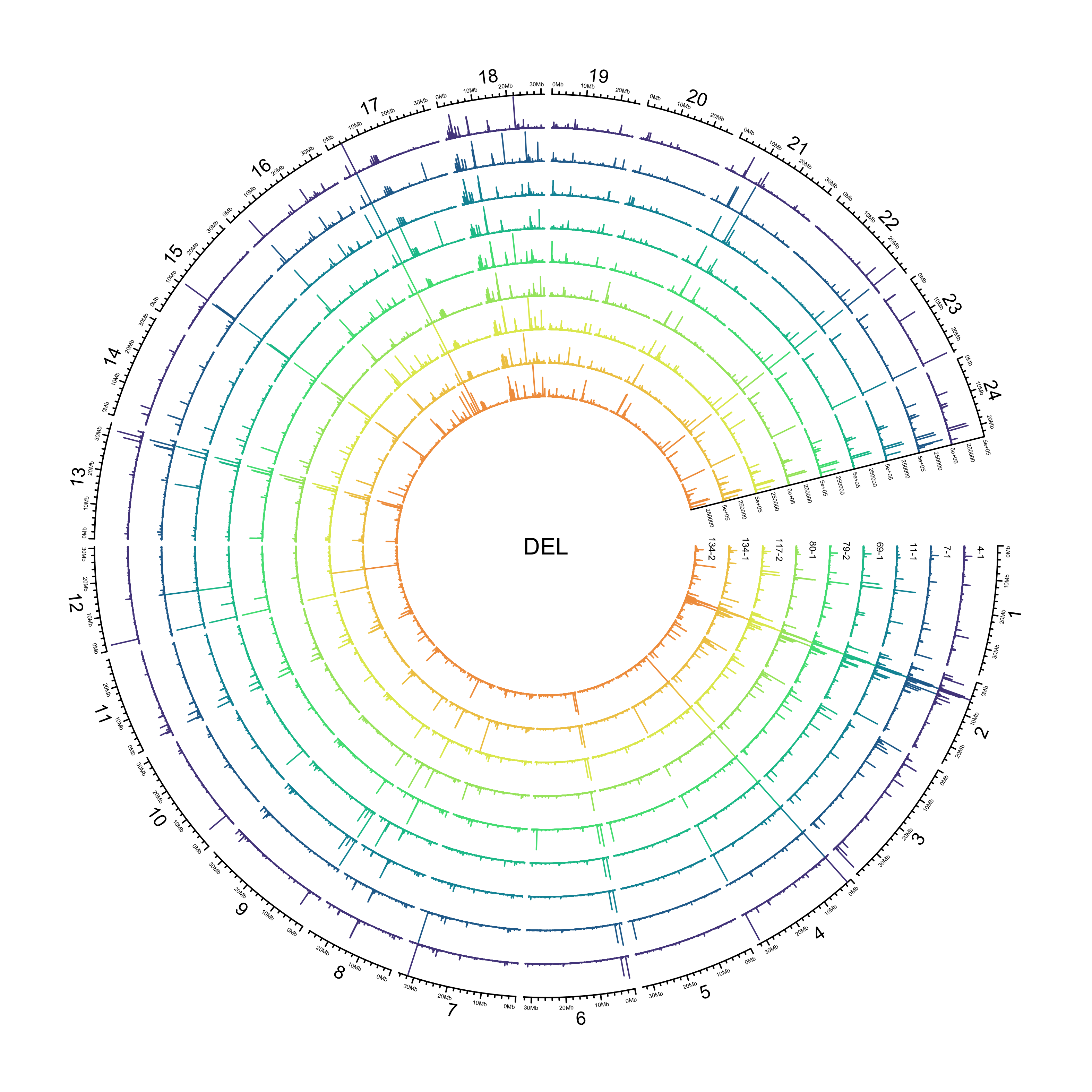
Circos plots
SVGs become very large (~80 MB). Hence PNG.
DEL
sv_dels = sv_df %>%
  dplyr::filter(DATASET == "polished",
                SVTYPE == "DEL") %>%
  dplyr::select(CHROM, POS, END, SAMPLE, LN) %>%
  dplyr::mutate(SAMPLE = factor(SAMPLE, levels = ont_samples_pol)) %>%
  split(., f = .$SAMPLE)
out_plot = here::here("docs/plots/sv_analysis/20210325_sv_dels_lines.png")
png(out_plot,
    width = 20,
    height = 20,
    units = "cm",
    res = 400)

# Get max value for `ylim`
max_len = max(sapply(sv_dels, function(sample) max(sample$LN)))
max_len = round.choose(max_len, 1e5, dir = 1)

# Choose palette
pal = grDevices::colorRampPalette(pal_smrarvo)(length(sv_dels))

# Set parameters
## Decrease cell padding from default c(0.02, 1.00, 0.02, 1.00)
circos.par(cell.padding = c(0, 0, 0, 0),
           track.margin = c(0, 0),
           gap.degree = c(rep(1, nrow(chroms) - 1), 14))
# Initialize plot
circos.initializeWithIdeogram(chroms,
                              plotType = c("axis", "labels"),
                              major.by = 1e7,
                              axis.labels.cex = 0.25*par("cex"))

# Print label in center
text(0, 0, "DEL")

counter = 0
lapply(sv_dels, function(sample) {
  # Set counter
  counter <<- counter + 1
  # Create track
  circos.genomicTrack(sample,
    panel.fun = function(region, value, ...) {
      circos.genomicLines(region,
                          value,
                          type = "h",
                          col = pal[counter],
                          cex = 0.05)
  },
  track.height = 0.07,
  bg.border = NA,
  ylim = c(0, max_len))

  # Add SV length y-axis label
  circos.yaxis(side = "right",
             at = c(2.5e5, max_len),
             labels.cex = 0.25*par("cex"),
             tick.length = 2
             )


  # Add SAMPLE y-axis label
  circos.text(2e6, 2.5e5,
              labels = names(sv_dels)[counter],
              sector.index = "chr1",
              cex = 0.4*par("cex"))
})


circos.clear()

dev.off()
knitr::include_graphics(out_plot)
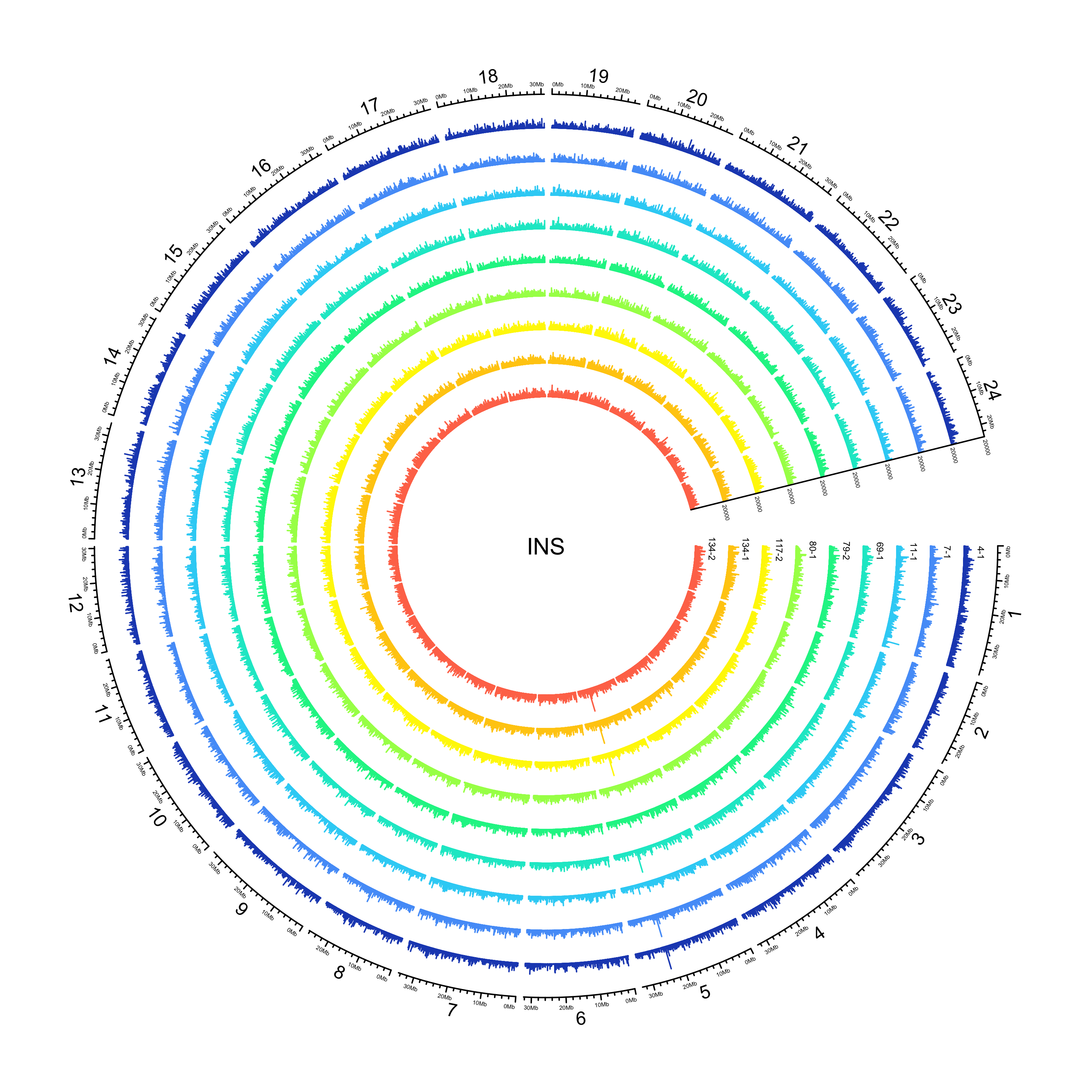
INS
NOTE: 25982/351996 insertions have an END that is less than POS. Make the END the same as POS for the purposes of plotting their location.
sv_ins = sv_df %>%
  dplyr::filter(DATASET == "polished",
                SVTYPE == "INS") %>%
  dplyr::select(CHROM, POS, END, SAMPLE, LN) %>%
  # Factorise SAMPLE to order
  dplyr::mutate(SAMPLE = factor(SAMPLE, levels = ont_samples_pol)) %>%
  # if END is less than POS, make it the same as POS
  dplyr::mutate(END = dplyr::if_else(END < POS, POS, END)) %>%
#  dplyr::slice_sample(n = 10000) %>%
  split(., f = .$SAMPLE)
out_plot = here::here("docs/plots/sv_analysis/20210325_sv_ins_lines.png")
png(out_plot,
    width = 20,
    height = 20,
    units = "cm",
    res = 400)

# Get max value for `ylim`
max_len = max(sapply(sv_ins, function(sample) max(sample$LN)))
max_len = round.choose(max_len, 1e4, dir = 1)

# Choose palette
pal = fishualize::fish(n = length(sv_ins), option = "Cirrhilabrus_solorensis")

# Set parameters
## Decrease cell padding from default c(0.02, 1.00, 0.02, 1.00)
circos.par(cell.padding = c(0, 0, 0, 0),
           track.margin = c(0, 0),
           gap.degree = c(rep(1, nrow(chroms) - 1), 14))
# Initialize plot
circos.initializeWithIdeogram(chroms,
                              plotType = c("axis", "labels"),
                              major.by = 1e7,
                              axis.labels.cex = 0.25*par("cex"))

# Print label in center
text(0, 0, "INS")

counter = 0
lapply(sv_ins, function(sample) {
  # Set counter
  counter <<- counter + 1
  # Create track
  circos.genomicTrack(sample,
    panel.fun = function(region, value, ...) {
      circos.genomicLines(region,
                          value,
                          type = "h",
                          col = pal[counter],
                          cex = 0.05)
  },
  track.height = 0.07,
  bg.border = NA,
  ylim = c(0, max_len))

  # Add SV length y-axis label
  circos.yaxis(side = "right",
             at = c(2.5e5, max_len),
             labels.cex = 0.25*par("cex"),
             tick.length = 2
             )


  # Add SAMPLE y-axis label
  circos.text(2e6, 1e4,
              labels = names(sv_ins)[counter],
              sector.index = "chr1",
              cex = 0.4*par("cex"))
})


circos.clear()

dev.off()
knitr::include_graphics(out_plot)
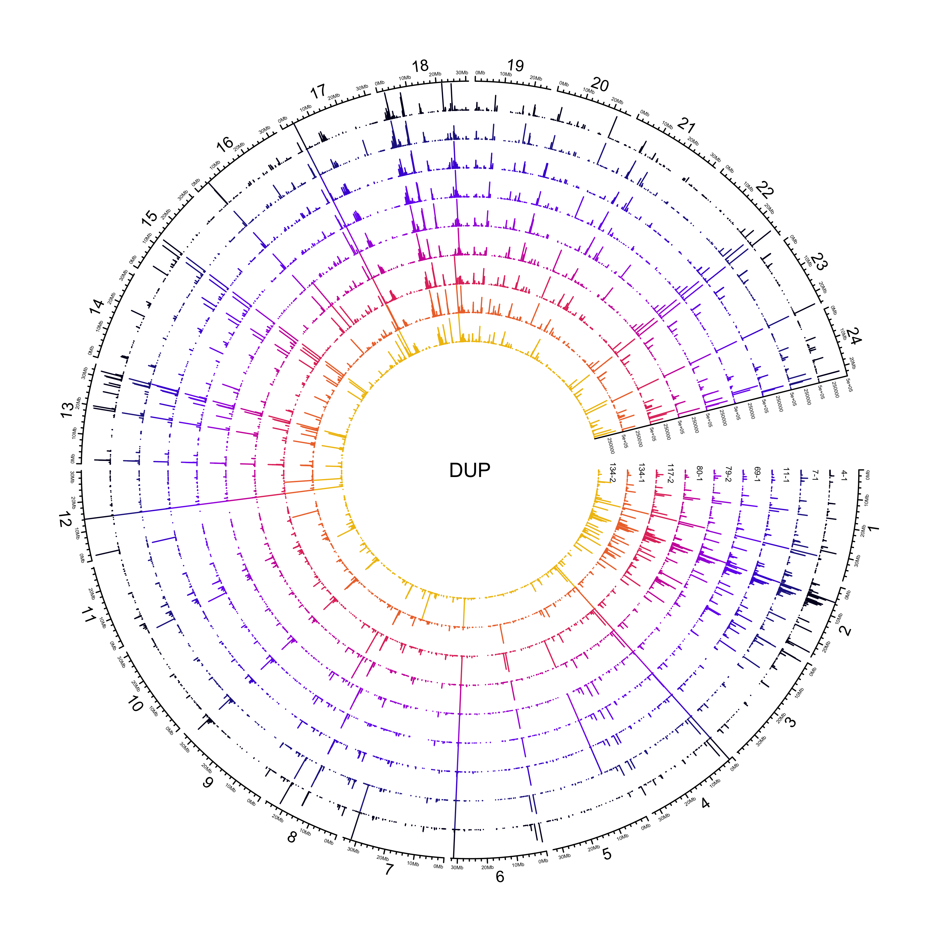
DUP
NOTE: 307/26823 duplications have an END that is less than POS. Make the END the same as POS.
sv_dups = sv_df %>%
  dplyr::filter(DATASET == "polished",
                SVTYPE == "DUP") %>%
  dplyr::select(CHROM, POS, END, SAMPLE, LN) %>%
  dplyr::mutate(SAMPLE = factor(SAMPLE, levels = ont_samples_pol)) %>%
  # if END is less than POS, make it the same as POS
  dplyr::mutate(END = dplyr::if_else(END < POS, POS, END)) %>%
#  dplyr::slice_sample(n = 10000) %>%
  split(., f = .$SAMPLE)
out_plot = here::here("docs/plots/sv_analysis/20210325_sv_dups_lines.png")
png(out_plot,
    width = 20,
    height = 20,
    units = "cm",
    res = 400)

# Get max value for `ylim`
max_len = max(sapply(sv_dups, function(sample) max(sample$LN)))
max_len = round.choose(max_len, 1e5, dir = 1)

# Choose palette
pal = fishualize::fish(n = length(sv_dups), option = "Gramma_loreto")

# Set parameters
## Decrease cell padding from default c(0.02, 1.00, 0.02, 1.00)
circos.par(cell.padding = c(0, 0, 0, 0),
           track.margin = c(0, 0),
           gap.degree = c(rep(1, nrow(chroms) - 1), 14))
# Initialize plot
circos.initializeWithIdeogram(chroms,
                              plotType = c("axis", "labels"),
                              major.by = 1e7,
                              axis.labels.cex = 0.25*par("cex"))

# Print label in center
text(0, 0, "DUP")

counter = 0
lapply(sv_dups, function(sample) {
  # Set counter
  counter <<- counter + 1
  # Create track
  circos.genomicTrack(sample,
    panel.fun = function(region, value, ...) {
      circos.genomicLines(region,
                          value,
                          type = "h",
                          col = pal[counter],
                          cex = 0.05)
  },
  track.height = 0.07,
  bg.border = NA,
  ylim = c(0, max_len))

  # Add SV length y-axis label
  circos.yaxis(side = "right",
             at = c(2.5e5, max_len),
             labels.cex = 0.25*par("cex"),
             tick.length = 2
             )


  # Add SAMPLE y-axis label
  circos.text(2e6, 2.5e5,
              labels = names(sv_dups)[counter],
              sector.index = "chr1",
              cex = 0.4*par("cex"))
})


circos.clear()

dev.off()
knitr::include_graphics(out_plot)
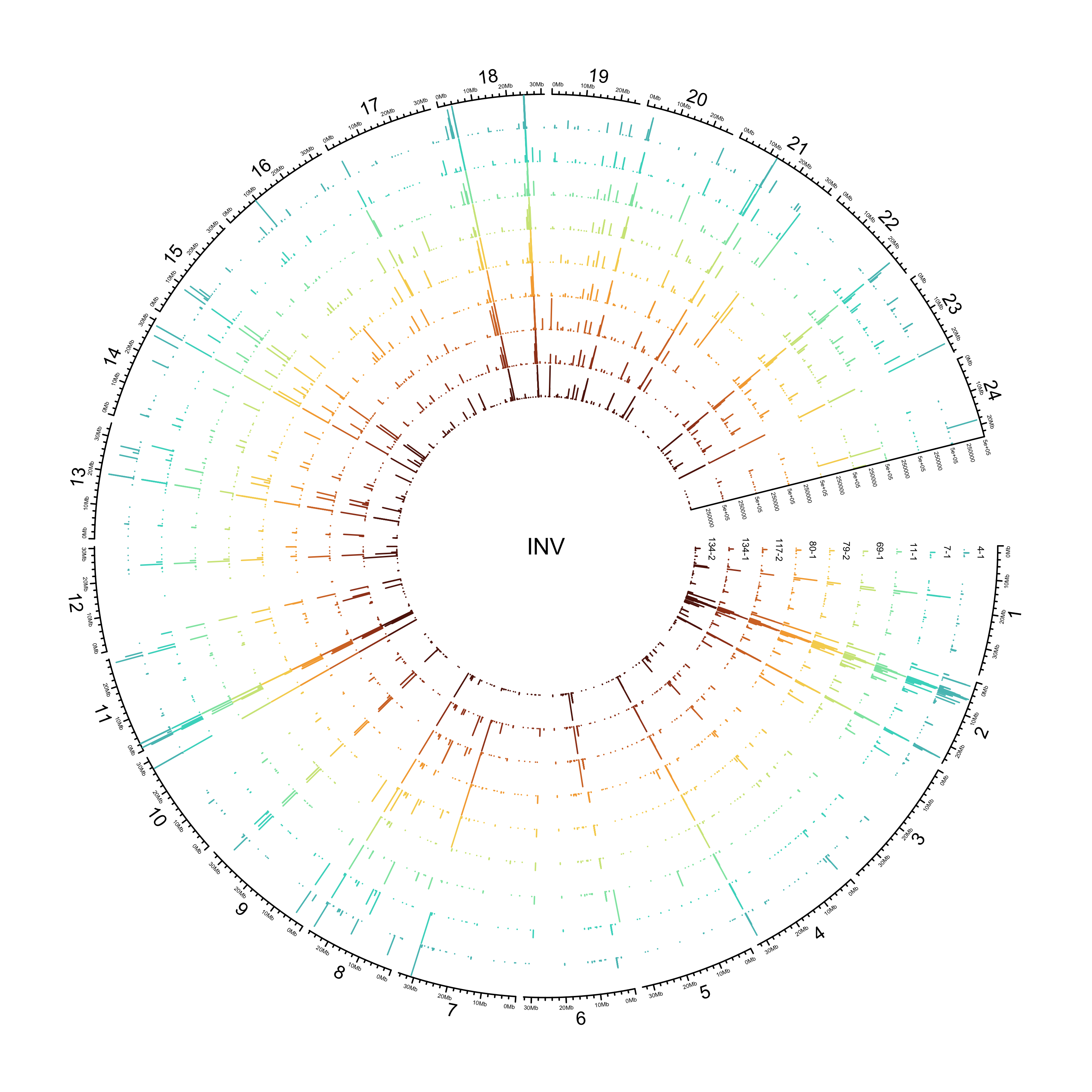
INV
sv_invs = sv_df %>%
  dplyr::filter(DATASET == "polished",
                SVTYPE == "INV") %>%
  dplyr::select(CHROM, POS, END, SAMPLE, LN) %>%
  dplyr::mutate(SAMPLE = factor(SAMPLE, levels = ont_samples_pol)) %>%
  # if END is less than POS, make it the same as POS
#  dplyr::mutate(END = dplyr::if_else(END < POS, POS, END)) %>%
#  dplyr::slice_sample(n = 10000) %>%
  split(., f = .$SAMPLE)
out_plot = here::here("docs/plots/sv_analysis/20210325_sv_invs_lines.png")
png(out_plot,
    width = 20,
    height = 20,
    units = "cm",
    res = 400)

# Get max value for `ylim`
max_len = max(sapply(sv_invs, function(sample) max(sample$LN)))
max_len = round.choose(max_len, 1e5, dir = 1)

# Choose palette
pal = fishualize::fish(n = length(sv_invs), option = "Lepomis_megalotis")

# Set parameters
## Decrease cell padding from default c(0.02, 1.00, 0.02, 1.00)
circos.par(cell.padding = c(0, 0, 0, 0),
           track.margin = c(0, 0),
           gap.degree = c(rep(1, nrow(chroms) - 1), 14))
# Initialize plot
circos.initializeWithIdeogram(chroms,
                              plotType = c("axis", "labels"),
                              major.by = 1e7,
                              axis.labels.cex = 0.25*par("cex"))

# Print label in center
text(0, 0, "INV")

counter = 0
lapply(sv_invs, function(sample) {
  # Set counter
  counter <<- counter + 1
  # Create track
  circos.genomicTrack(sample,
    panel.fun = function(region, value, ...) {
      circos.genomicLines(region,
                          value,
                          type = "h",
                          col = pal[counter],
                          cex = 0.05)
  },
  track.height = 0.07,
  bg.border = NA,
  ylim = c(0, max_len))

  # Add SV length y-axis label
  circos.yaxis(side = "right",
             at = c(2.5e5, max_len),
             labels.cex = 0.25*par("cex"),
             tick.length = 2
             )


  # Add SAMPLE y-axis label
  circos.text(2e6, 2.5e5,
              labels = names(sv_invs)[counter],
              sector.index = "chr1",
              cex = 0.4*par("cex"))
})


circos.clear()

dev.off()
knitr::include_graphics(out_plot)
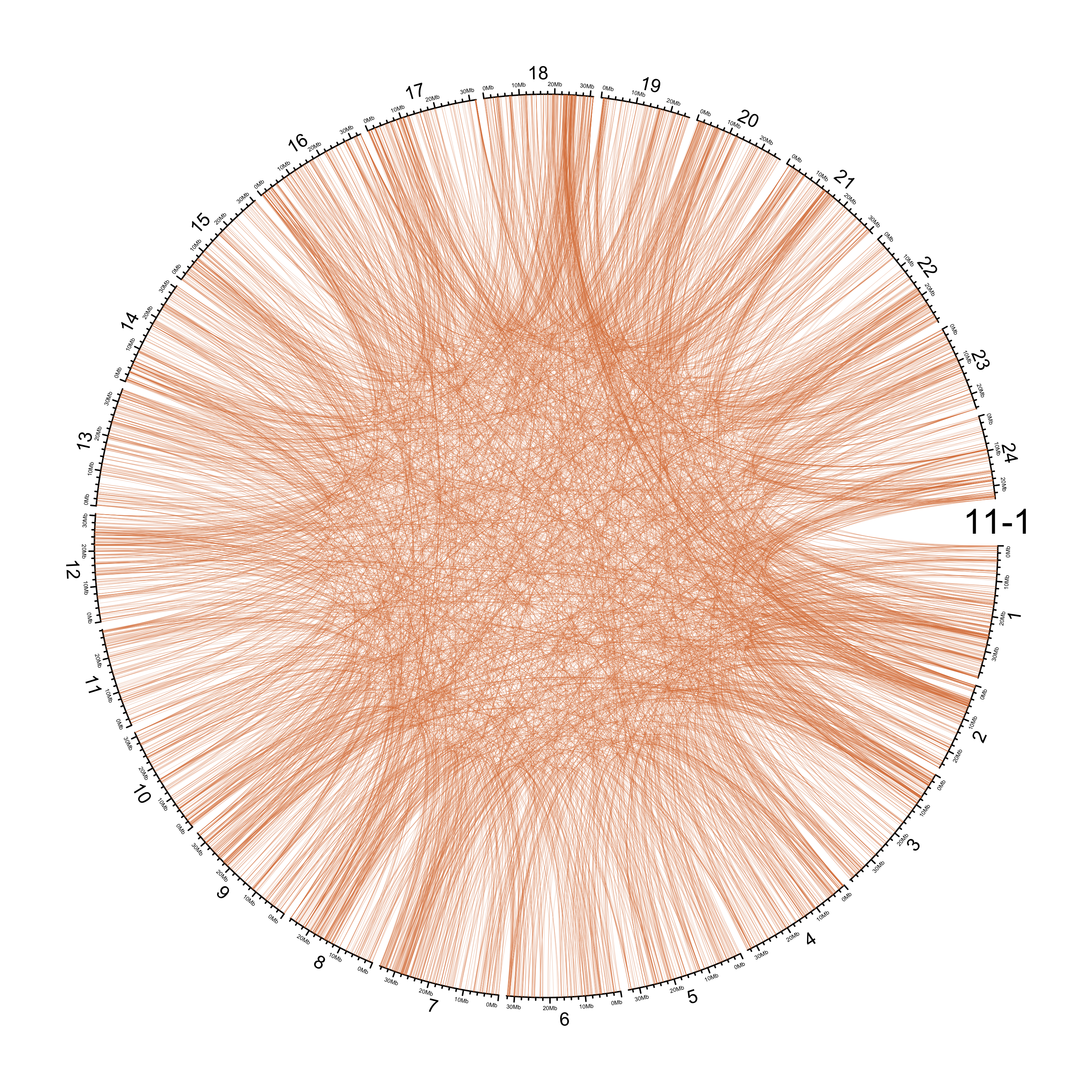
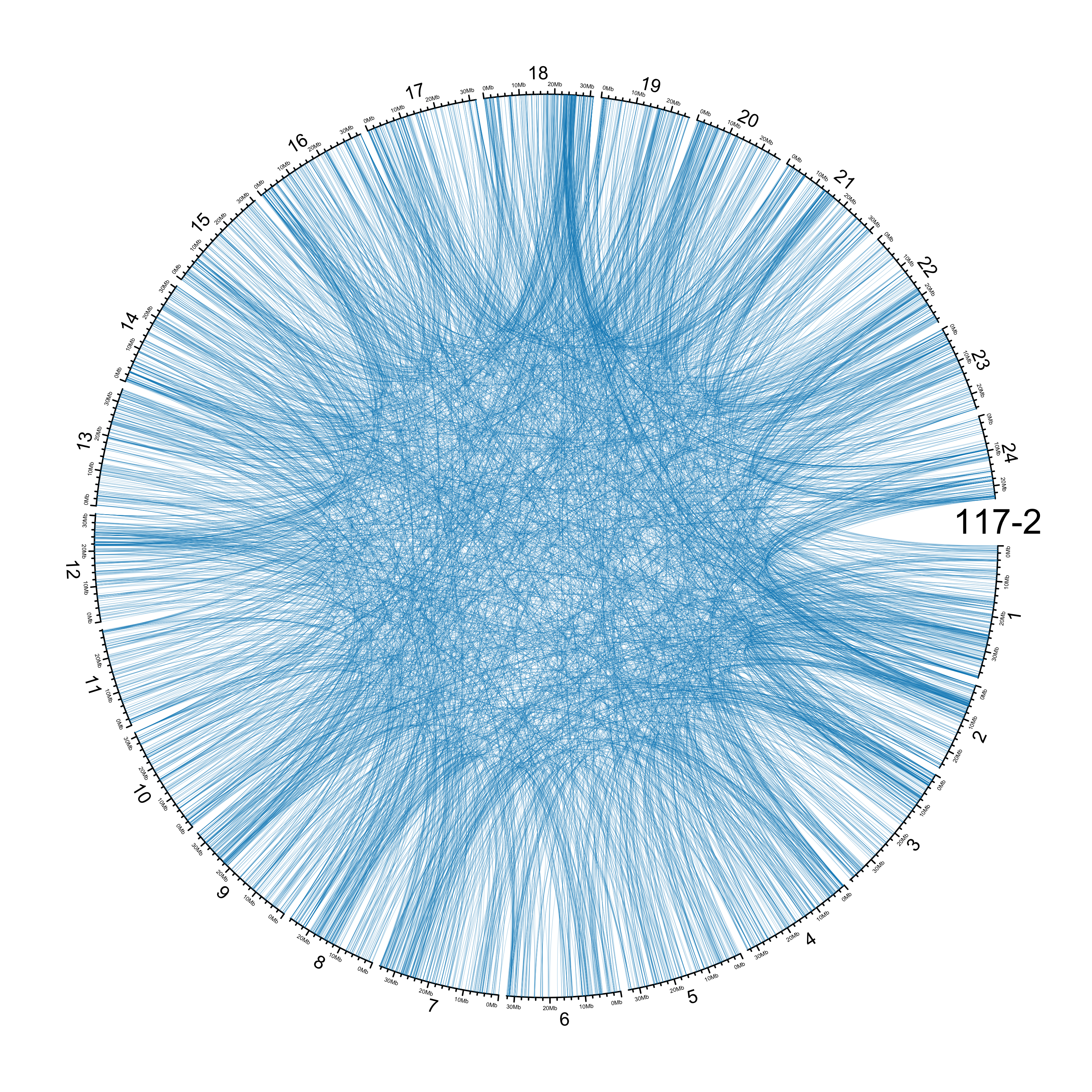
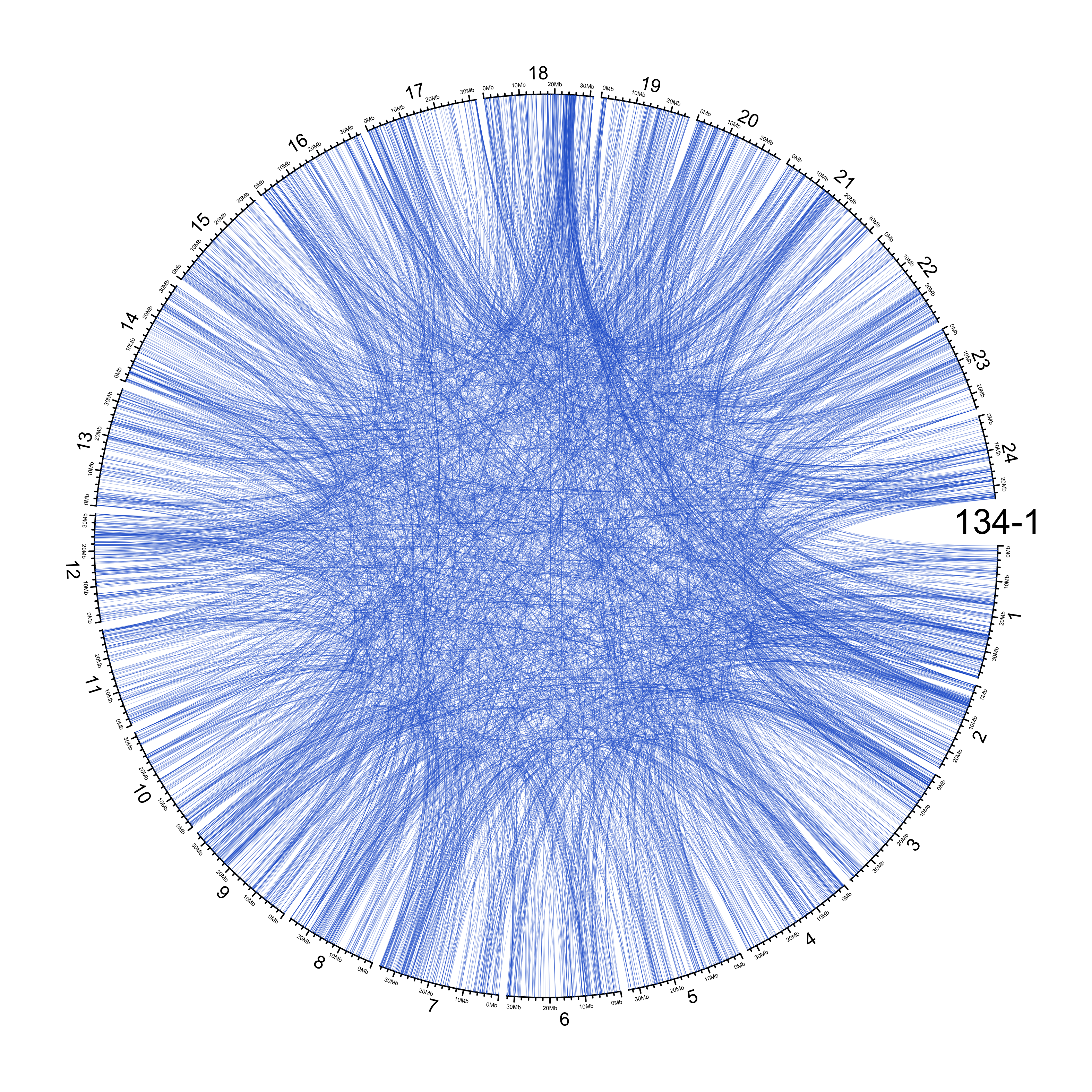
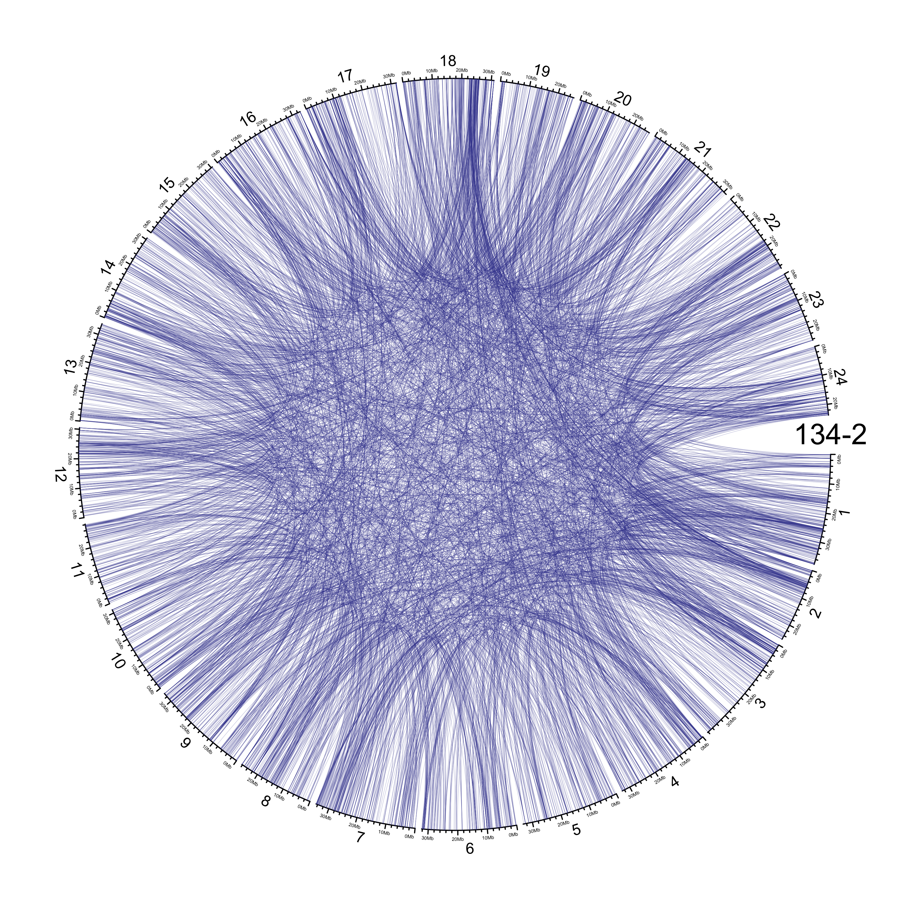
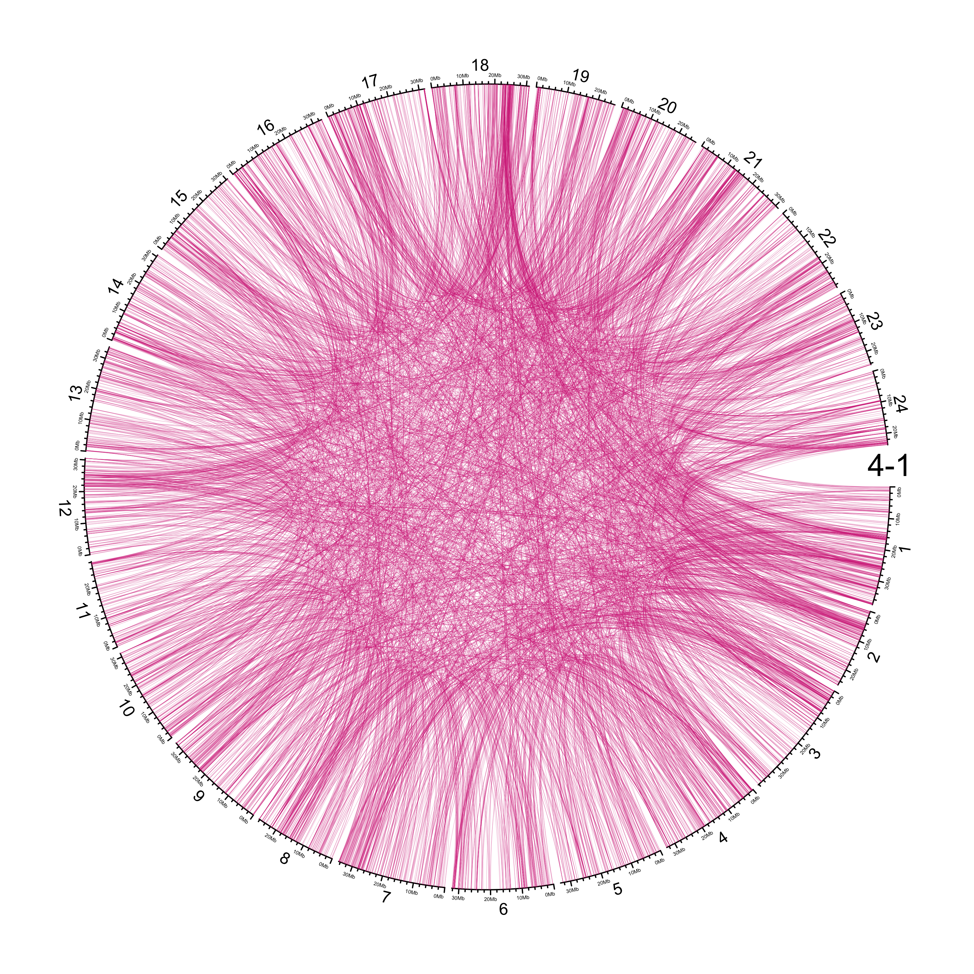
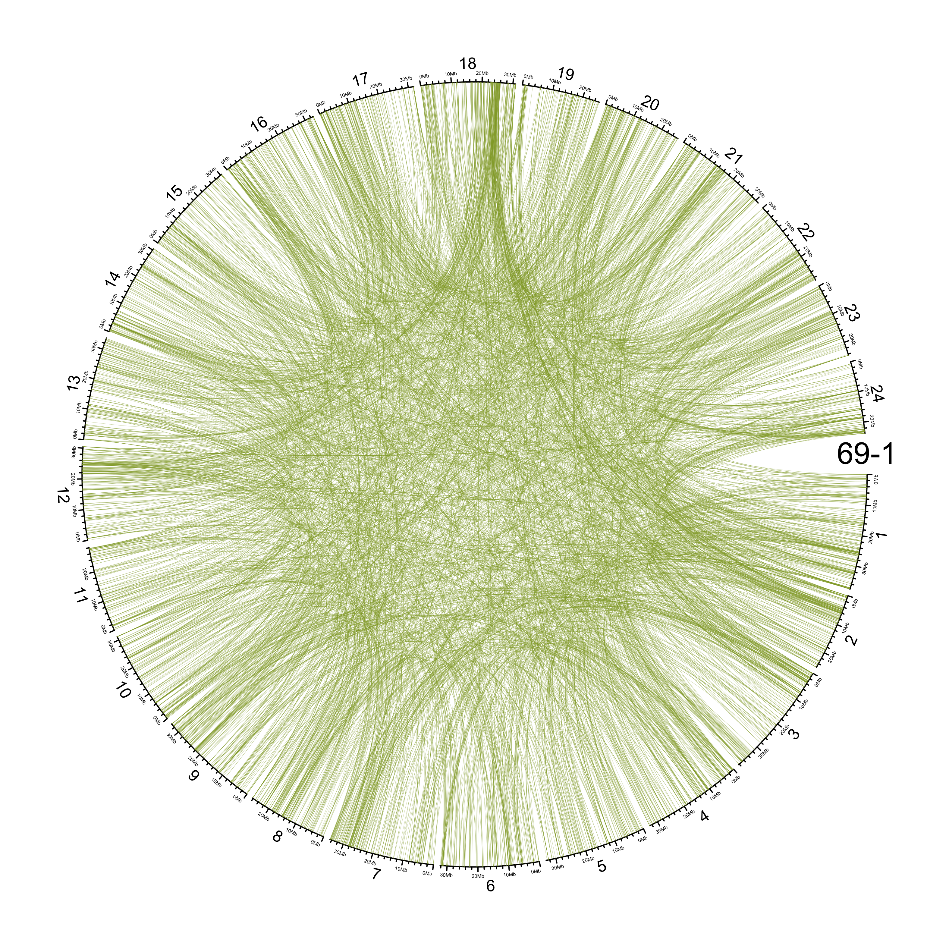
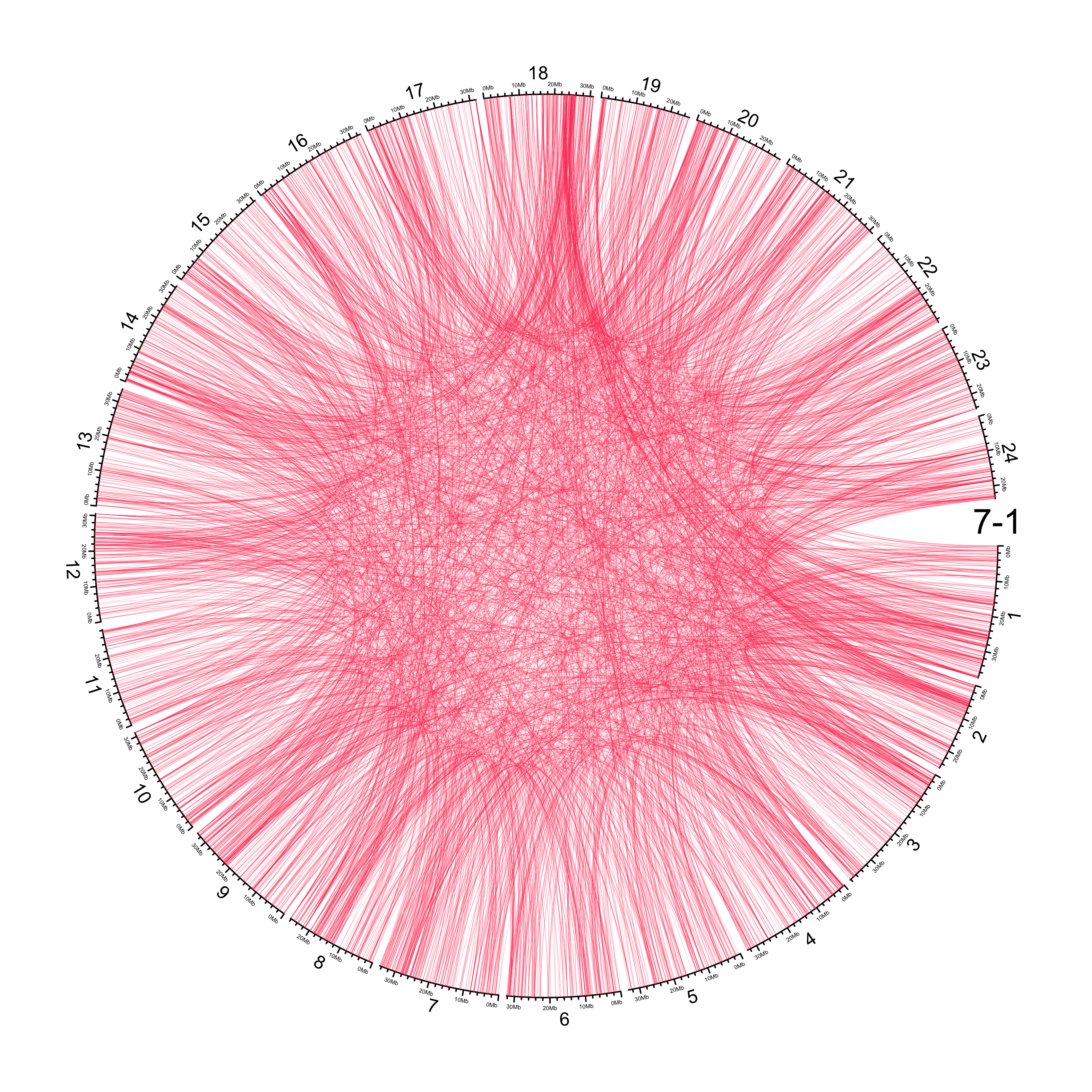
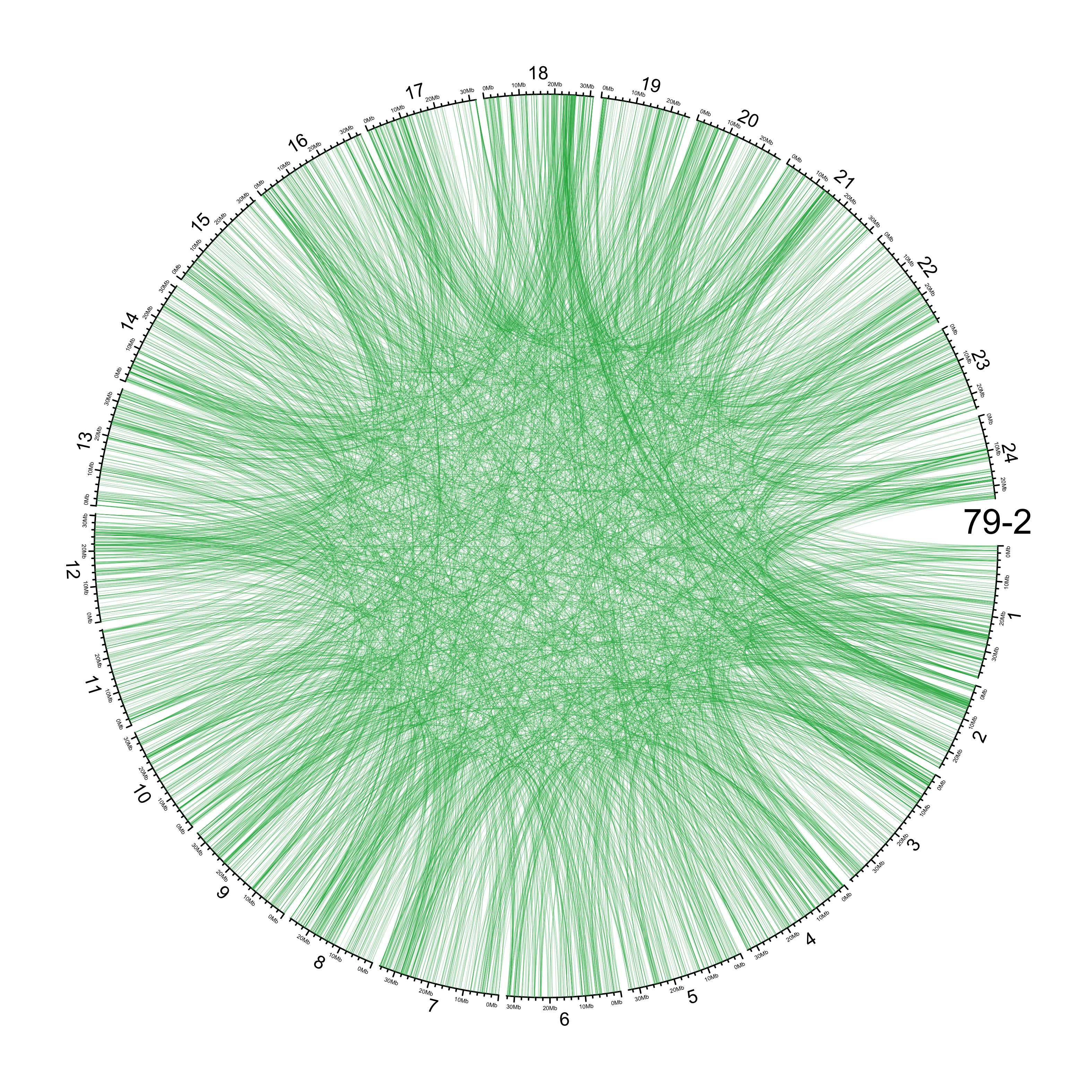
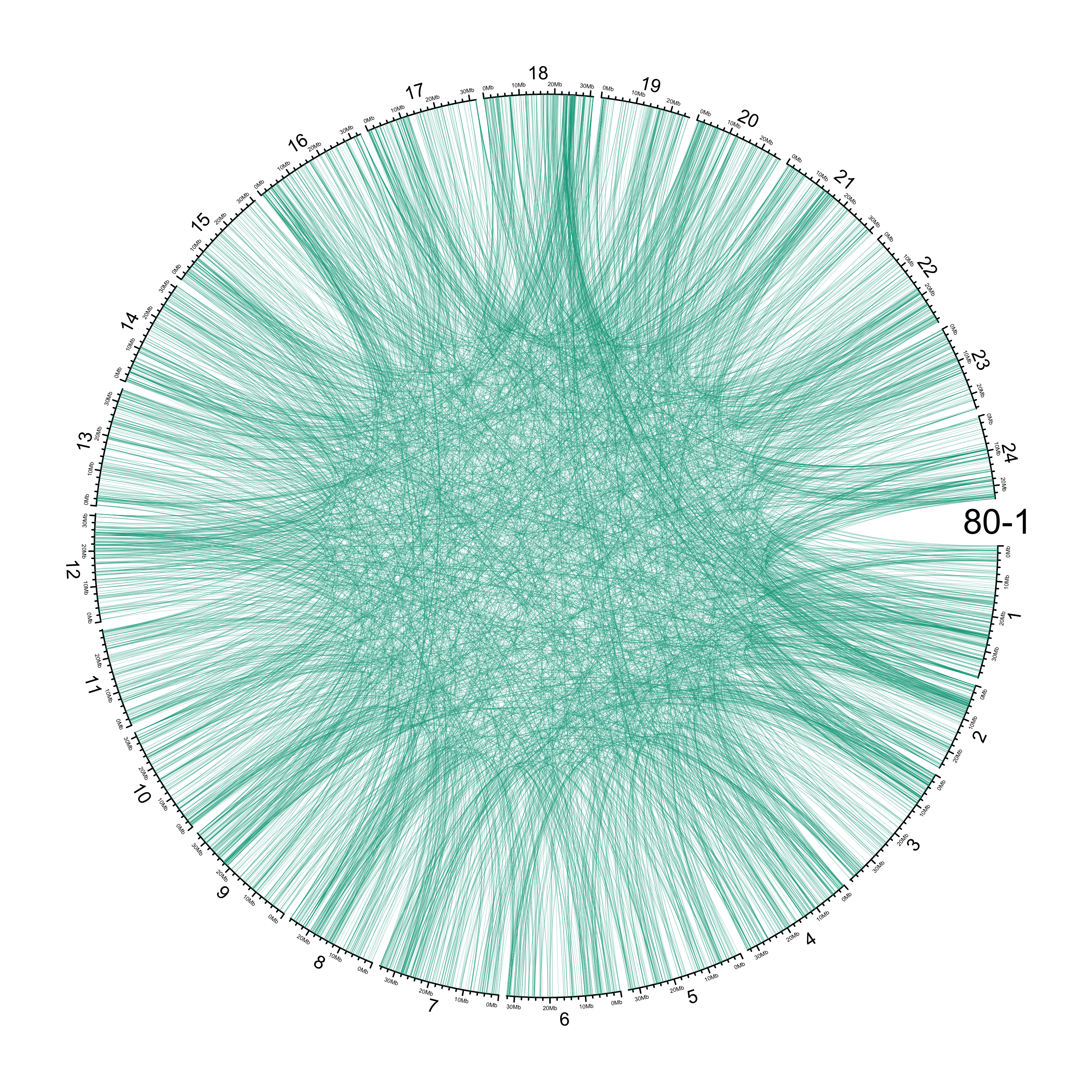
TRA
out_dir = here::here("docs/plots/sv_analysis/20210326_tras")
in_samples = ont_samples_pol
pal = fishualize::fish(n = length(in_samples), option = "Scarus_quoyi")
counter = 0
lapply(in_samples, function(TARGET_SAMPLE){
  # Set counter
  counter <<- counter + 1

  # Get data
  sv_tras = sv_df %>%
    dplyr::filter(DATASET == "polished",
                  SVTYPE == "TRA") %>%
    # test with single sample
    dplyr::filter(SAMPLE == TARGET_SAMPLE) %>%
    # select key columns
    dplyr::select(CHROM, POS, ALT, CHR2, END)

  loc_1 = sv_tras %>%
    dplyr::select(CHROM, START = POS, END = POS)

  loc_2 = sv_tras %>%
    dplyr::select(CHROM = CHR2, START = END, END = END) %>%
    dplyr::mutate(CHROM = paste("chr", CHROM, sep = ""))

  out_plot = here::here(out_dir, paste(TARGET_SAMPLE, ".png", sep = ""))

  png(out_plot,
      width = 20,
      height = 20,
      units = "cm",
      res = 400)

  # Set parameters
  ## Decrease cell padding from default c(0.02, 1.00, 0.02, 1.00)
  circos.par(cell.padding = c(0, 0, 0, 0),
             track.margin = c(0, 0),
             gap.degree = c(rep(1, nrow(chroms) - 1), 6))
  # Initialize plot
  circos.initializeWithIdeogram(chroms,
                                plotType = c("axis", "labels"),
                                major.by = 1e7,
                                axis.labels.cex = 0.25*par("cex"))

  circos.genomicLink(loc_1, loc_2,
                     col = grDevices::adjustcolor(pal[counter], alpha.f = 0.4),
                     lwd = .25*par("lwd"),
                     border = NA)

  circos.text(0, 0,
              labels = TARGET_SAMPLE,
              sector.index = "chr1",
              facing = "clockwise",
              adj = c(0.5, -0.5),
              cex = 1.5*par("cex"))

  circos.clear()

  dev.off()

})
knitr::include_graphics(list.files(out_dir, full.names = T))
Main figure
final_svtype = ggdraw() +
  draw_image(here::here("docs/plots/sv_analysis/20210325_sv_dels_lines.png"),
           x = 0, y = 0, width = 1, height = .75, scale = 1.12) +
  draw_plot(svtype_counts_plot,
            x = 0, y = .75, width = .5, height = .25) +
  draw_plot(svlen_counts_plot,
            x = .5, y = .75, width =.5, height = .25) +
  draw_plot_label(label = c("A", "B", "C"), size = 25,
                  x = c(0, .5, 0), y = c(1, 1, .75),color = "#4f0943")

final_svtype

ggsave(here::here("docs/plots/sv_analysis/20210325_sv_main.png"),
       device = "png",
       dpi = 400,
       units = "cm",
       width = 30,
       height = 42)
How many unique SVs?
# Total count of unique SVs
length(unique(sv_df_pol$ID))
## [1] 143326
# By SV Type
sv_df_pol %>%
  dplyr::filter(!duplicated(ID)) %>%
  dplyr::group_by(SVTYPE) %>%
  dplyr::count()
## # A tibble: 5 × 2
## # Groups:   SVTYPE [5]
##   SVTYPE     n
##   <chr>  <int>
## 1 DEL    67052
## 2 DUP     5690
## 3 INS    59990
## 4 INV     1356
## 5 TRA     9238
Distribution of singletons across chromosomes
sv_sings %>%
  dplyr::mutate(CHROM = gsub("chr", "", CHROM),
                CHROM = factor(CHROM, levels = 1:24)) %>%
  dplyr::group_by(CHROM, SAMPLE) %>%
  dplyr::summarise(N = n()) %>%
  dplyr::ungroup() %>%
  ggplot() +
    geom_col(aes(CHROM, N, fill = CHROM)) +
    facet_wrap(~SAMPLE) +
    theme_bw() +
    theme(axis.text.x = element_text(size = 5)) +
    guides(fill = "none") +
    ggtitle("Singletons")
## `summarise()` has grouped output by 'CHROM'. You can override using the `.groups` argument.

ggsave(here::here(plots_dir, "20210325_singleton_counts_by_chr.png"),
       device = "png",
       width = 20,
       height = 9.375,
       units = "cm",
       dpi = 400)
Distribution of non-singletons across chromosomes
sv_df %>%
  dplyr::filter(DATASET == "polished") %>%
  # Exclude singletons
  dplyr::anti_join(sv_sings, by = c("CHROM", "POS", "LN")) %>%
  # Order CHROM
  dplyr::mutate(CHROM = gsub("chr", "", CHROM),
                CHROM = factor(CHROM, levels = 1:24)) %>%
  dplyr::group_by(CHROM) %>%
  dplyr::summarise(N = n()) %>%
  tidyr::drop_na() %>%
  dplyr::ungroup() %>%
  ggplot() +
    geom_col(aes(CHROM, N, fill = CHROM)) +
    theme_bw() +
    guides(fill = "none") +
    ggtitle("Non-singletons (i.e. shared by at least two lines)")

ggsave(here::here(plots_dir, "20210325_shared_svs_by_chr.png"),
       device = "png",
       width = 15,
       height = 9.375,
       units = "cm",
       dpi = 400)
Investigate interesting variants
Large insertion on chr 5
# Get locations of insertions longer than 300 kb on chr 17
sv_ins %>%
  dplyr::bind_rows() %>%
  dplyr::filter(CHROM == "chr5" & LN > 10000)
## # A tibble: 6 × 5
##   CHROM      POS      END SAMPLE    LN
##   <chr>    <int>    <int> <fct>  <int>
## 1 chr5  23770083 23770083 4-1    13649
## 2 chr5  23770083 23770083 7-1    13649
## 3 chr5  23770083 23770083 69-1   13649
## 4 chr5  23770083 23770083 117-2  13649
## 5 chr5  23770083 23770083 134-1  13649
## 6 chr5  23770083 23770083 134-2  13649
grep "23770083"  ../sv_analysis/vcfs/ont_raw_with_seq_rehead_per_sample/4-1.vcf
# Returns a sequence that is only 1000 bases long?
#5  23770083    51143   N   <INS>   .   PASS    SUPP=12;SUPP_VEC=111111111111;SVLEN=13649;SVTYPE=INS;SVMETHOD=SURVIVOR1.0.7;CHR2=5;END=23770083;CIPOS=0,0;CIEND=0,0;STRANDS=-+GT:PSV:LN:DR:ST:QV:TY:ID:RAL:AAL:CO   1/1:NA:13649:0,6:-+:.:INS:51143:N:TATGAGGGGCTTTATAAGACATTATTTATTCTGAACCATTCACATTCATACATTCTGCTCTCACAGTCATATACTCTTTCGCATACATATATTCTCTTACGCATCCATATATTCTCTCTCACATTCATACATTCTTTGCTCTCACAGTCATATATACTCTCTTTCGCATACATATATTCTCACTTGCACATTCATATATTCTCTCTCGCATGCATATATATTACTTTTACACATACATACATTCTCACTCTATTGTCACTCTTAAAAAGAATGTATGTGTGAAAGACAAGTATATATGAACGTGTGAGGAAGAGTTTATATGTGTGTGTGTGAGAGAGGAGTATGCATGAAACGGAAGTGACTTTGCATGAAAAGGAAGGCACTTGAATGAAAAGAAGGCACTTTGCATGAAACGGAAGGCAGATGATTTCTCGTGCTCTGATTGGACGAGAGGCCGCCACCTCCCATTTTGAACACACTCTAAACCCTATCACTTGTACTGACTCATAACTATTAAGGTTACACAACTCAAATGTCATTTCGTAGTTGGATTCAACTATAAAGTATTAAGCTCTATCAAGATTTTTTCAAATTTAACTTAACAGTGTTAAATATTTTAAAGCTTATTTGTATCTAGCACTCTAAAATTTTAAGATTCCTGAAGTAGCGTCATGATCGTCACACACTGGTGGGAGGGTCTTTCGTTTTCTACGTTAGCTCAGGTGGCCATGTTGGATTTGTCAATGCGAGTATGCGACGTTTTGAAATTGAAAGTCGAGCATTTTATTTTTCTGCAAAGCATTTCGCTCCCGCTTCAAGACGCCCAACTCGGGTTTTTTCATCCGCCTCATCGCTGATGGTGCCGTCTTGTCTTCAGCCCTGATTTAAATTTGGTAAGTATCGTTCATGGTTTATTTTGAACGAATGTTTAAAATGCTCTTATACCACCGTAAATGTGGTTTACTGTTGTTTAAACATATGTGTGTTATGATTGTTTTA:5_23770083-5_23770083
Explore shared variation between 131-1 and HdrR/HNI
Key files:
- 131-1 assembly:
/hps/research1/birney/users/adrien/indigene/analyses/indigene_nanopore_DNA/graph_genome_analysis/individual_assemblies/131-1_F4_clean.fa
HNI reference: /hps/research1/birney/users/adrien/indigene/analyses/indigene_nanopore_DNA/graph_genome_analysis/references/Oryzias_latipes_HNI_clean.fa
You may also like to do against HDrR: /hps/research1/birney/users/adrien/indigene/analyses/indigene_nanopore_DNA/graph_genome_analysis/references/Oryzias_latipes_HDRR_clean.fa
Run minigraph
container=../sing_conts/minigraph.sif
in_fasta=/hps/research1/birney/users/adrien/indigene/analyses/indigene_nanopore_DNA/graph_genome_analysis/individual_assemblies/131-1_F4_clean.fa
ref_pref=/hps/research1/birney/users/adrien/indigene/analyses/indigene_nanopore_DNA/graph_genome_analysis/references/Oryzias_latipes
out_dir=../sv_analysis/pafs

mkdir -p $out_dir

for target_ref in $(echo HNI HDRR ) ; do
  bsub \
    -M 30000 \
    -n 16 \
    -o ../log/20210322_minigraph_$target_ref.out \
    -e ../log/20210322_minigraph_$target_ref.err \
    """
    singularity exec $container \
      /minigraph/minigraph $in_fasta $ref_pref\_$target_ref\_clean.fa \
        > $out_dir/MIKK_131-1_to_$target_ref.paf
    """ ;
done

# Flip other way around
## Usage: minigraph [options] <target.gfa> <query.fa> [...]
## So use the reference as the target, 131-1 as the query
for target_ref in $(echo HNI HDRR ) ; do
  bsub \
    -M 20000 \
    -n 16 \
    -o ../log/20210322_minigraph_flipped_$target_ref.out \
    -e ../log/20210322_minigraph_flipped_$target_ref.err \
    """
    singularity exec $container \
      /minigraph/minigraph $ref_pref\_$target_ref\_clean.fa $in_fasta \
        > $out_dir/$target_ref\_to_MIKK_131-1.paf
    """ ;
done

data_dir=data/sv_analysis/pafs
mkdir -p $data_dir && cp $out_dir/*131-1.paf $data_dir
Documentation for paf format: https://github.com/lh3/miniasm/blob/master/PAF.md
Read in data
in_dir = here::here("data/sv_analysis/pafs")

in_files = list.files(in_dir, full.names = T)
names(in_files) = basename(in_files) %>%
  stringr::str_split(., pattern = "_", simplify = T) %>%
  subset(select = 1)

col_names = c("QUERY_SEQ_NAME",
              "QUERY_SEQ_LEN",
              "QUERY_START",
              "QUERY_END",
              "STRAND",
              "TARGET_NAME",
              "TARGET_LEN",
              "TARGET_START",
              "TARGET_END",
              "RESIDUE_MATCHES",
              "BLOCK_LENGTH",
              "MAPPING_QUALITY")

pafs = purrr::map(in_files, function(x) {
  readr::read_tsv(x,
                  col_names = col_names,
                  col_types = "ciiicciiiiii-----")
})
Circos
Process intrgression data
in_file = here::here("data/introgression/abba_sliding_final_131-1/1000000_250.txt")
# Read in data
df_intro = readr::read_csv(in_file) %>%
  dplyr::arrange(p1, p2, scaffold, start)

# Convert fd to 0 if D < 0
df_intro$fd = ifelse(df_intro$D < 0,
               0,
               df_intro$fd)

# Change names
df_intro = df_intro %>%
  dplyr::mutate(p2 = recode(df_intro$p2, hdrr = "HdrR", hni = "HNI", hsok = "HSOK"))

# Get mean of javanicus and melastigma
df_intro = df_intro %>%
  pivot_wider(id_cols = c(scaffold, start, end, mid, p2), names_from = p1, values_from = fd) %>%
  # get mean of melastigma/javanicus
  dplyr::mutate(mean_fd = rowMeans(dplyr::select(., melastigma, javanicus), na.rm = T)) %>%
  dplyr::arrange(p2, scaffold, start) %>%
  dplyr::select(scaffold, mid_1 = mid, mid_2 = mid, mean_fd, p2) %>%
  dplyr::mutate(scaffold = paste("chr", scaffold, sep ="")) %>%
  split(., f = .$p2)
Process alignment data
pal_length = 1000
# Get palette
pal_viridis = viridis(pal_length)
names(pal_viridis) = 1:pal_length

pal_inferno = inferno(pal_length)
names(pal_inferno) = 1:pal_length

counter = 0
# Process data
paf_clean = pafs %>%
  purrr::map(function(x) {
    # Set counter
    counter <<- counter + 1
    # Select palette
    if (names(pafs)[counter] == "HDRR"){
      pal_chosen = pal_viridis
    } else if (names(pafs)[counter] == "HNI"){
      pal_chosen = pal_inferno
    }
    # Clean data
    x %>%
      dplyr::mutate(TARGET_MID = round(TARGET_START + ((TARGET_END - TARGET_START) / 2)),
                    CHROM = stringr::str_replace_all(TARGET_NAME, c("HDRR_" = "chr", "HNI_" = "chr")),
                    CHROM = factor(CHROM, levels = paste("chr", 1:24, sep = "")),
                    PERCENT_MATCHED = RESIDUE_MATCHES / BLOCK_LENGTH,
                    LOG_BLOCK_LENGTH = log10(BLOCK_LENGTH),
                    COL = cut(PERCENT_MATCHED, breaks = 1000, labels = F),
                    COL = dplyr::recode(COL, !!!pal_chosen)) %>%
#      dplyr::slice_sample(n = 1000) %>%
      dplyr::arrange(CHROM, TARGET_START)
})
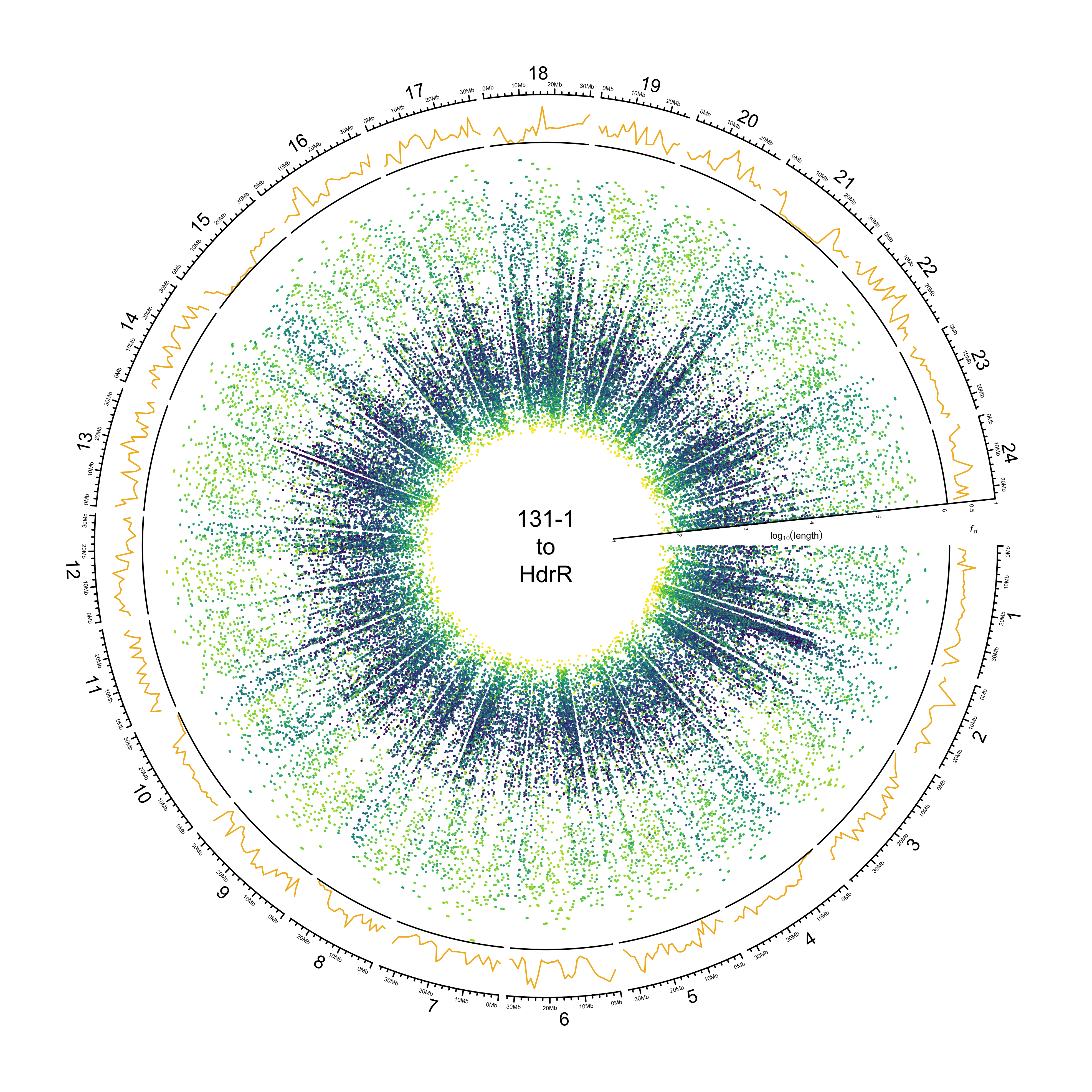
HdrR
out_plot = here::here("docs/plots/sv_analysis/20210323_circos_hdrr_alignments.png")
png(out_plot,
    width = 20,
    height = 20,
    units = "cm",
    res = 500)

ylim = c(1, 6.05)
target_line = "HdrR"

# Set parameters
## Decrease cell padding from default c(0.02, 1.00, 0.02, 1.00)
circos.par(cell.padding = c(0, 0, 0, 0),
           track.margin = c(0, 0),
           gap.degree = c(rep(1, nrow(chroms) - 1), 6))
# Initialize plot
circos.initializeWithIdeogram(chroms,
                              plotType = c("axis", "labels"),
                              major.by = 1e7,
                              axis.labels.cex = 0.25*par("cex"))

# Print label in center
text(0, 0, "131-1\nto\nHdrR")

###############
# Introgression
###############

circos.genomicTrack(df_intro[[target_line]],
    panel.fun = function(region, value, ...){
      circos.genomicLines(region,
                          value[[1]],
                          col = pal_abba[[target_line]])
      # Add baseline
      circos.xaxis(h = "bottom",
                   labels = F,
                   major.tick = F)
    },
    track.height = 0.1,
    bg.border = NA,
    ylim = c(0, 1))


# Add axis for introgression
circos.yaxis(side = "right",
           at = c(.5, 1),
           labels.cex = 0.25*par("cex"),
           tick.length = 2
           )

# Add y-axis label for introgression
circos.text(0, 0.5,
            labels = expression(italic(f[d])),
            sector.index = "chr1",
            facing = "clockwise",
            adj = c(.5, -1.5),
            cex = 0.4*par("cex"))

###############
# Alignments
###############

circos.genomicTrack(paf_clean[[stringr::str_to_upper(target_line)]] %>%
                      dplyr::select(CHROM, TARGET_START, TARGET_END,
                                    LOG_BLOCK_LENGTH, PERCENT_MATCHED, COL),
    panel.fun = function(region, value, ...){
      circos.genomicLines(region,
                          value[[1]],
                          type = "segment",
                          col = value[[3]],
                          lwd = 1.5)
}, track.height = 0.7,
   bg.border = NA,
   ylim = ylim
   )

# Add SV length y-axis label
circos.yaxis(side = "right",
           at = 1:6,
           labels.cex = 0.25*par("cex"),
           tick.length = 2
           )

# Add  y-axis label
circos.text(0, 3.75,
            labels = expression(log[10](length)),
            sector.index = "chr1",
            facing = "clockwise",
            adj = c(0.5, -0.5),
            cex = 0.4*par("cex"))

circos.clear()

dev.off()
knitr::include_graphics(out_plot)
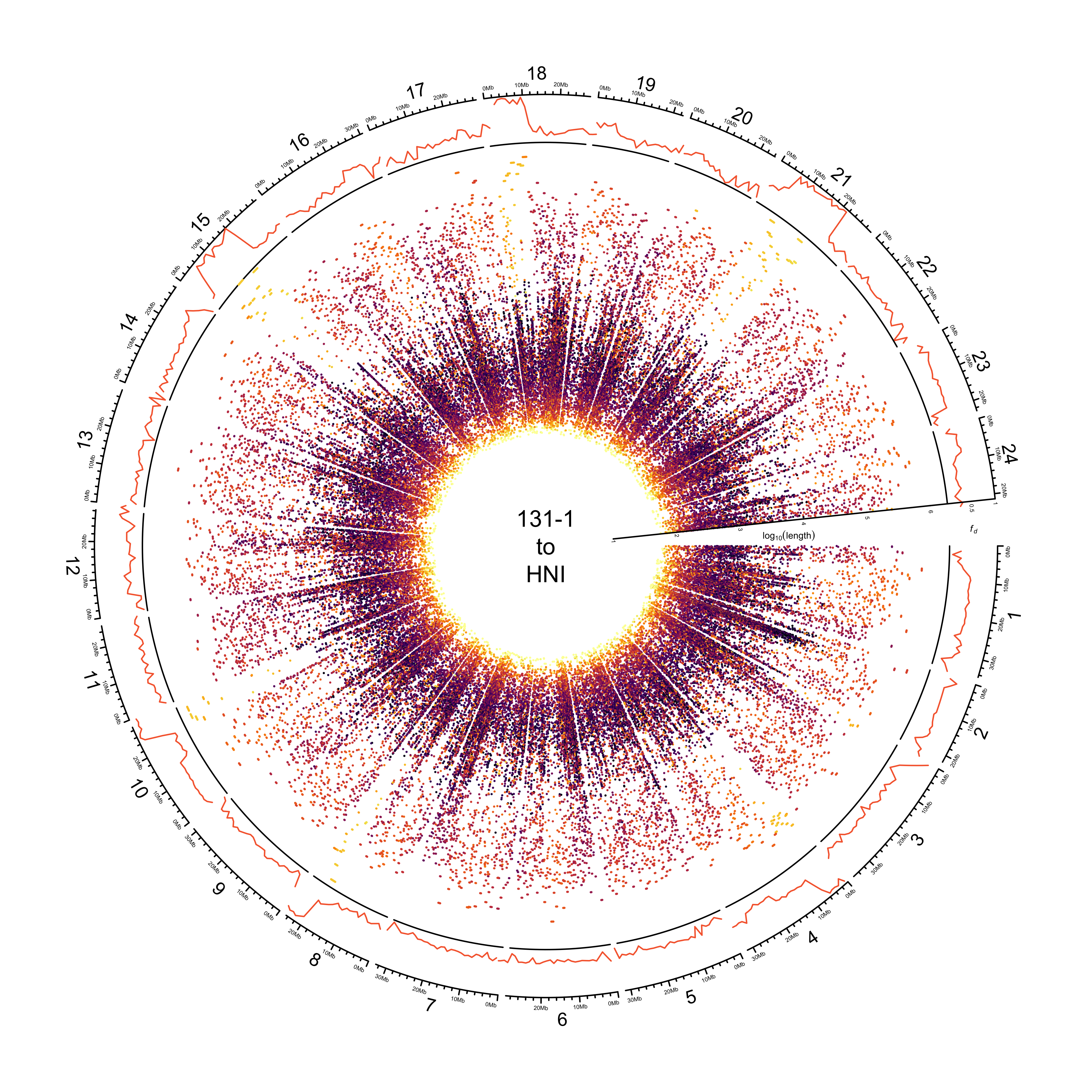
HNI
Create chroms file for HNI
# Get chrs
grep ">" ../refs/Oryzias_latipes_hni.ASM223471v1.dna.toplevel.fa | cut -f1 -d" " | sed 's/>//g' > tmp1
# Get lengths
grep ">" ../refs/Oryzias_latipes_hni.ASM223471v1.dna.toplevel.fa | cut -f3 -d' ' | cut -f5 -d':' > tmp2
# Paste and send to file
paste tmp1 tmp2 > data/Oryzias_latipes_hni.ASM223471v1.dna.toplevel.fa_chr_counts.txt
# Clean up
rm tmp1 tmp2
# Read in chromosome data
chroms_hni = read.table(here::here("data/Oryzias_latipes_hni.ASM223471v1.dna.toplevel.fa_chr_counts.txt")) %>%
  dplyr::select(chr = V1, end = V2) %>%
  dplyr::mutate(chr = paste("chr", chr, sep = ""),
                start = 0,
                end = as.numeric(end)) %>%
  dplyr::select(chr, start, end)
out_plot = here::here("docs/plots/sv_analysis/20210323_circos_hni_alignments.png")
png(out_plot,
    width = 20,
    height = 20,
    units = "cm",
    res = 500)

ylim = c(1, 6.27)

target_line = "HNI"

# Set parameters
## Decrease cell padding from default c(0.02, 1.00, 0.02, 1.00)
circos.par(cell.padding = c(0, 0, 0, 0),
           track.margin = c(0, 0),
           gap.degree = c(rep(1, nrow(chroms_hni) - 1), 6))
# Initialize plot
circos.initializeWithIdeogram(chroms_hni,
                              plotType = c("axis", "labels"),
                              major.by = 1e7,
                              axis.labels.cex = 0.25*par("cex"))

# Print label in center
text(0, 0, "131-1\nto\nHNI")

###############
# Introgression
###############

circos.genomicTrack(df_intro[[target_line]],
    panel.fun = function(region, value, ...){
      circos.genomicLines(region,
                          value[[1]],
                          col = pal_abba[[target_line]])
      # Add baseline
      circos.xaxis(h = "bottom",
                   labels = F,
                   major.tick = F)
    },
    track.height = 0.1,
    bg.border = NA,
    ylim = c(0, 1))


# Add axis for introgression
circos.yaxis(side = "right",
           at = c(.5, 1),
           labels.cex = 0.25*par("cex"),
           tick.length = 2
           )

# Add y-axis label for introgression
circos.text(0, 0.5,
            labels = expression(italic(f[d])),
            sector.index = "chr1",
            facing = "clockwise",
            adj = c(.5, -1.5),
            cex = 0.4*par("cex"))

###############
# Alignments
###############

circos.genomicTrack(paf_clean[[target_line]] %>%
                      dplyr::select(CHROM, TARGET_START, TARGET_END,
                                    LOG_BLOCK_LENGTH, PERCENT_MATCHED, COL),
    panel.fun = function(region, value, ...){
      circos.genomicLines(region,
                          value[[1]],
                          type = "segment",
                          col = value[[3]],
                          lwd = 1.5)
}, track.height = 0.7,
   bg.border = NA,
   ylim = ylim
   )

# Add SV length y-axis label
circos.yaxis(side = "right",
           at = 1:6,
           labels.cex = 0.25*par("cex"),
           tick.length = 2
           )

# Add  y-axis label
circos.text(0, 3.75,
            labels = expression(log[10](length)),
            sector.index = "chr1",
            facing = "clockwise",
            adj = c(0.5, -0.5),
            cex = 0.4*par("cex"))

circos.clear()

dev.off()
knitr::include_graphics(out_plot)
Histograms showing distribution of identity
paf_clean %>%
  dplyr::bind_rows(.id = "REFERENCE") %>%
  dplyr::mutate(REFERENCE = dplyr::recode(REFERENCE, HDRR = "HdrR")) %>%
  ggplot() +
    geom_density(aes(PERCENT_MATCHED, fill = REFERENCE)) +
    facet_wrap(~REFERENCE) +
    theme_bw() +
    guides(fill = "none") +
    scale_fill_manual(values = pal_abba) +
    xlab("BLAST identity")

ggsave(here::here(plots_dir, "20210323_131-1_identity_density.png"),
       device = "png",
       width = 20,
       height = 9.375,
       units = "cm",
       dpi = 400)
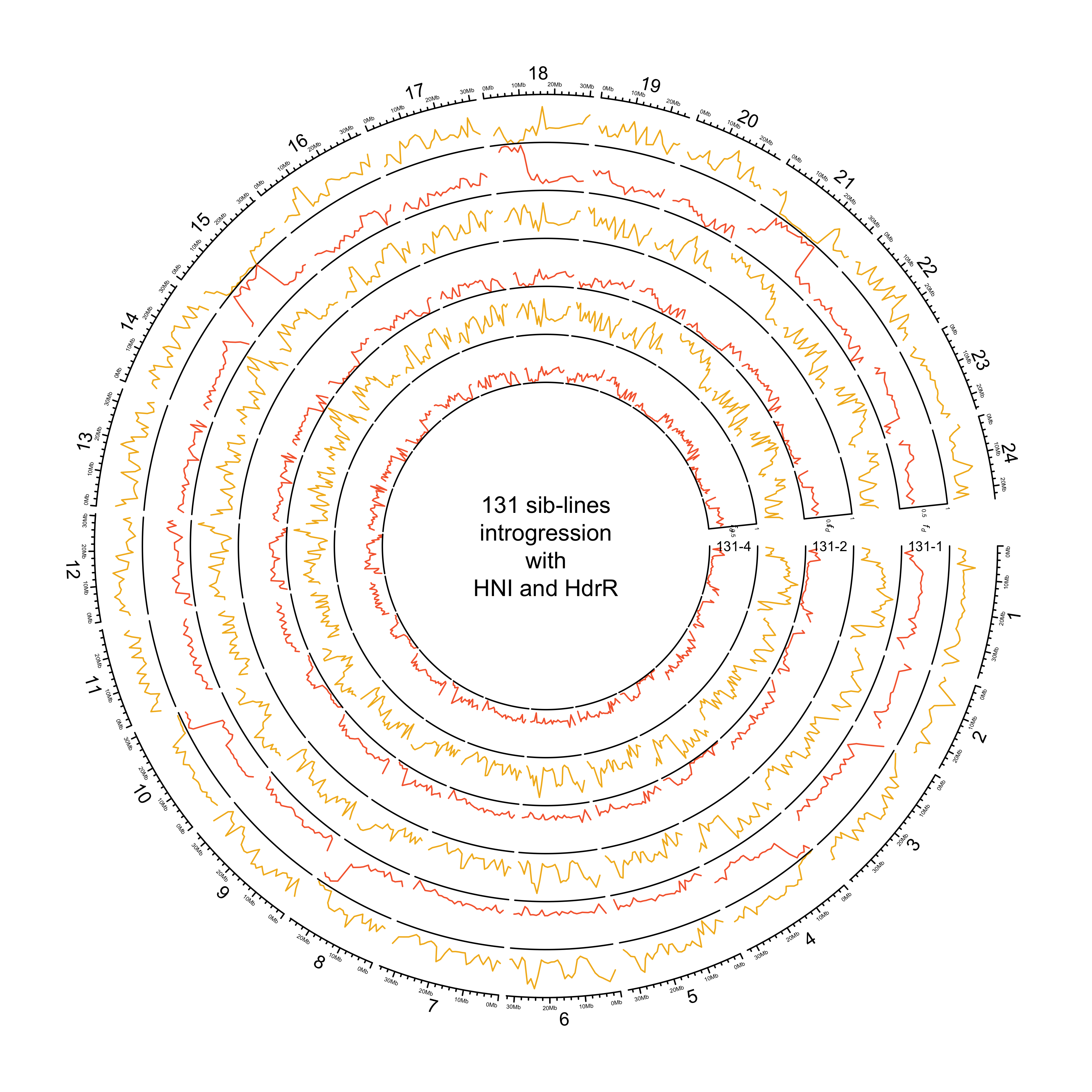
Get circos for all 131 sibling lines
in_dir = here::here("data/introgression/abba_sliding_final_131")

in_files = list.files(in_dir, full.names = T)
names(in_files) = basename(in_files) %>%
  stringr::str_split("_") %>%
  purrr::map_chr(~ purrr::pluck(.x, 1))

# Read and process data
list_131 = purrr::map(in_files, readr::read_csv) %>%
  map(~ .x %>%
        dplyr::arrange(p1, p2, scaffold, start) %>%
        dplyr::mutate(fd = if_else(D < 0, 0, fd),
                      p2 = recode(p2, hdrr = "HdrR", hni = "HNI", hsok = "HSOK")) %>%
        tidyr::pivot_wider(id_cols = c(scaffold, start, end, mid, p2), names_from = p1, values_from = fd) %>%
        # get mean of melastigma/javanicus
        dplyr::mutate(mean_fd = rowMeans(dplyr::select(., melastigma, javanicus), na.rm = T)) %>%
        dplyr::arrange(p2, scaffold, start) %>%
        dplyr::select(scaffold, mid_1 = mid, mid_2 = mid, mean_fd, p2) %>%
        dplyr::mutate(scaffold = paste("chr", scaffold, sep ="")) %>%
        split(., f = .$p2)
      )
HNI
out_plot = here::here("docs/plots/sv_analysis/20210324_circos_131_siblines_HNI.png")
png(out_plot,
    width = 20,
    height = 20,
    units = "cm",
    res = 500)

# Set parameters
## Decrease cell padding from default c(0.02, 1.00, 0.02, 1.00)
circos.par(cell.padding = c(0, 0, 0, 0),
           track.margin = c(0, 0),
           gap.degree = c(rep(1, nrow(chroms) - 1), 6))
# Initialize plot
circos.initializeWithIdeogram(chroms,
                              plotType = c("axis", "labels"),
                              major.by = 1e7,
                              axis.labels.cex = 0.25*par("cex"))

# Print label in center
text(0, 0, "131 sib-lines\nintrogression\nwith\nHNI")

###############
# Introgression
###############
counter = 0

purrr::map(list_131, function(sib_line){
  # Set counter
  counter <<- counter + 1

  circos.genomicTrack(sib_line[["HNI"]],
      panel.fun = function(region, value, ...){
        circos.genomicLines(region,
                            value[[1]],
                            col = pal_abba[["HNI"]])
        # Add baseline
        circos.xaxis(h = "bottom",
                     labels = F,
                     major.tick = F)
      },
      track.height = 0.1,
      bg.border = NA,
      ylim = c(0, 1))

  # Add axis for introgression
  circos.yaxis(side = "right",
             at = c(.5, 1),
             labels.cex = 0.25*par("cex"),
             tick.length = 2
             )

  # Add y-axis label for introgression
  circos.text(0, 0.5,
              labels = expression(italic(f[d])),
              sector.index = "chr1",
#              facing = "clockwise",
              adj = c(3, 0.5),
              cex = 0.4*par("cex"))

  # Add y-axis label for introgression
  circos.text(0, 0.5,
              labels = names(list_131)[counter],
              sector.index = "chr1",
              facing = "clockwise",
#              adj = c(.5, -1.5),
              cex = 0.6*par("cex"))
})

circos.clear()

dev.off()
knitr::include_graphics(out_plot)
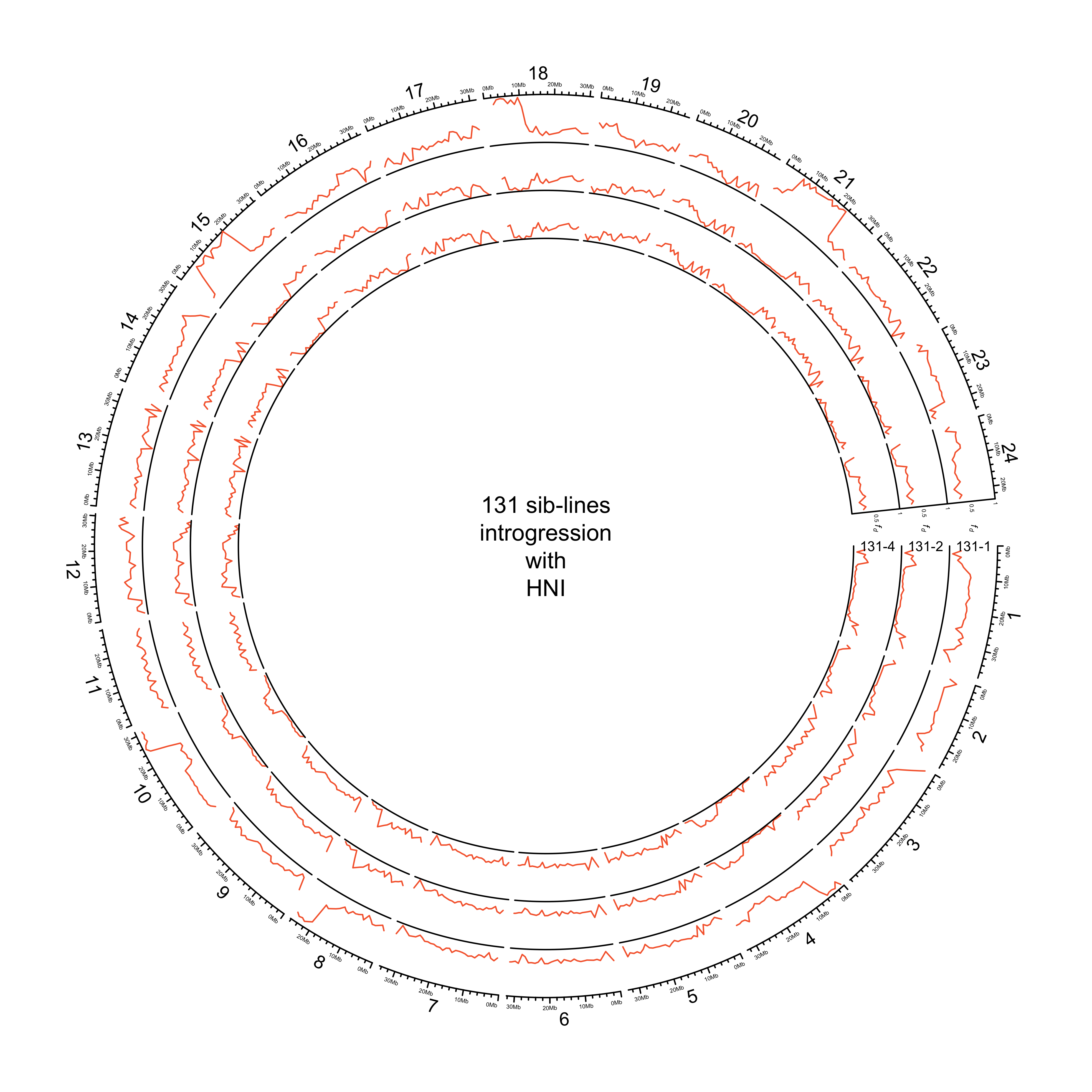
HdrR and HNI
out_plot = here::here("docs/plots/sv_analysis/20210324_circos_131_siblines_HdrR_HNI.png")
png(out_plot,
    width = 20,
    height = 20,
    units = "cm",
    res = 500)

# Set parameters
## Decrease cell padding from default c(0.02, 1.00, 0.02, 1.00)
circos.par(cell.padding = c(0, 0, 0, 0),
           track.margin = c(0, 0),
           gap.degree = c(rep(1, nrow(chroms) - 1), 6))
# Initialize plot
circos.initializeWithIdeogram(chroms,
                              plotType = c("axis", "labels"),
                              major.by = 1e7,
                              axis.labels.cex = 0.25*par("cex"))

# Print label in center
text(0, 0, "131 sib-lines\nintrogression\nwith\nHNI and HdrR")

###############
# Introgression
###############
counter = 0

purrr::map(list_131, function(sib_line){
  # Set counter
  counter <<- counter + 1

  circos.genomicTrack(sib_line[["HdrR"]],
      panel.fun = function(region, value, ...){
        circos.genomicLines(region,
                            value[[1]],
                            col = pal_abba[["HdrR"]])
        # Add baseline
        circos.xaxis(h = "bottom",
                     labels = F,
                     major.tick = F)
      },
      track.height = 0.1,
      bg.border = NA,
      ylim = c(0, 1))

  circos.genomicTrack(sib_line[["HNI"]],
      panel.fun = function(region, value, ...){
        circos.genomicLines(region,
                            value[[1]],
                            col = pal_abba[["HNI"]])
        # Add baseline
        circos.xaxis(h = "bottom",
                     labels = F,
                     major.tick = F)
      },
      track.height = 0.1,
      bg.border = NA,
      ylim = c(0, 1))


  # Add axis for introgression
  circos.yaxis(side = "right",
             at = c(.5, 1),
             labels.cex = 0.25*par("cex"),
             tick.length = 2
             )

  # Add y-axis label for introgression
  circos.text(0, 0.5,
              labels = expression(italic(f[d])),
              sector.index = "chr1",
#              facing = "clockwise",
              adj = c(3, 0.5),
              cex = 0.4*par("cex"))

  # Add y-axis label for introgression
  circos.text(0, 0.5,
              labels = names(list_131)[counter],
              sector.index = "chr1",
              facing = "clockwise",
#              adj = c(.5, -1.5),
              cex = 0.6*par("cex"))
})

circos.clear()

dev.off()
knitr::include_graphics(out_plot)
131-1 with HdrR, HNI and Kaga
Read in data
target_dir = here::here("data/introgression/abba_sliding_final_mikk/1000000_250")
files = list.files(target_dir, full.names = T)
names(files) = basename(files) %>%
  stringr::str_remove(".txt")

intro_mikk = purrr::map(files, function(x) x %>%
  readr::read_csv(.) %>%
  dplyr::mutate(fd = if_else(D < 0, 0, fd),
                p2 = factor(p2, levels = c("hdrr", "hni", "kaga", "hsok")),
                p2 = recode(p2, hdrr = "HdrR", hni = "HNI", hsok = "HSOK", kaga = "Kaga")) %>%
  tidyr::pivot_wider(id_cols = c(scaffold, start, end, mid, p2), names_from = p1, values_from = fd) %>%
  # get mean of melastigma/javanicus
  dplyr::mutate(mean_fd = rowMeans(dplyr::select(., melastigma, javanicus), na.rm = T)) %>%
  dplyr::arrange(p2, scaffold, start) %>%
  dplyr::select(scaffold, mid_1 = mid, mid_2 = mid, mean_fd, p2) %>%
  dplyr::mutate(scaffold = paste("chr", scaffold, sep ="")) %>%
  split(., f = .$p2)
)
out_plot = here::here("docs/plots/sv_analysis/20210330_circos_131-1_HdrR_HNI_Kaga_HSOK.png")
png(out_plot,
    width = 20,
    height = 20,
    units = "cm",
    res = 500)

# Set parameters
## Decrease cell padding from default c(0.02, 1.00, 0.02, 1.00)
circos.par(cell.padding = c(0, 0, 0, 0),
           track.margin = c(0, 0),
           gap.degree = c(rep(1, nrow(chroms) - 1), 6))
# Initialize plot
circos.initializeWithIdeogram(chroms,
                              plotType = c("axis", "labels"),
                              major.by = 1e7,
                              axis.labels.cex = 0.25*par("cex"))

# Print label in center
text(0, 0, "131-1 introgression\nwith\nHdrR, HNI,\nKaga and HSOK")

###############
# Introgression
###############
counter = 0

purrr::map(intro_mikk$`131_1`, function(P2){
  # Set counter
  counter <<- counter + 1

  circos.genomicTrack(P2,
      panel.fun = function(region, value, ...){
        circos.genomicLines(region,
                            value[[1]],
                            col = pal_abba[[names(intro_mikk$`131_1`[counter])]],
                            area = T,
                            border = karyoploteR::darker(pal_abba[[names(intro_mikk$`131_1`[counter])]]))
        # Add baseline
        circos.xaxis(h = "bottom",
                     labels = F,
                     major.tick = F)
      },
      track.height = 0.1,
      bg.border = NA,
      ylim = c(0, 1))

  # Add axis for introgression
  circos.yaxis(side = "right",
             at = c(.5, 1),
             labels.cex = 0.25*par("cex"),
             tick.length = 2
             )

  # Add y-axis label for introgression
  if (counter == 2) {
  circos.text(0, 0,
              labels = expression(italic(f[d])),
              sector.index = "chr1",
#              facing = "clockwise",
              adj = c(3, 0.5),
              cex = 0.4*par("cex"))
  }

  # Add y-axis label for introgression
  circos.text(0, 0.5,
              labels = names(intro_mikk$`131_1`)[counter],
              sector.index = "chr1",
              facing = "clockwise",
              adj = c(.5, 0),
              cex = 0.6*par("cex"))
})

circos.clear()

dev.off()
knitr::include_graphics(out_plot)
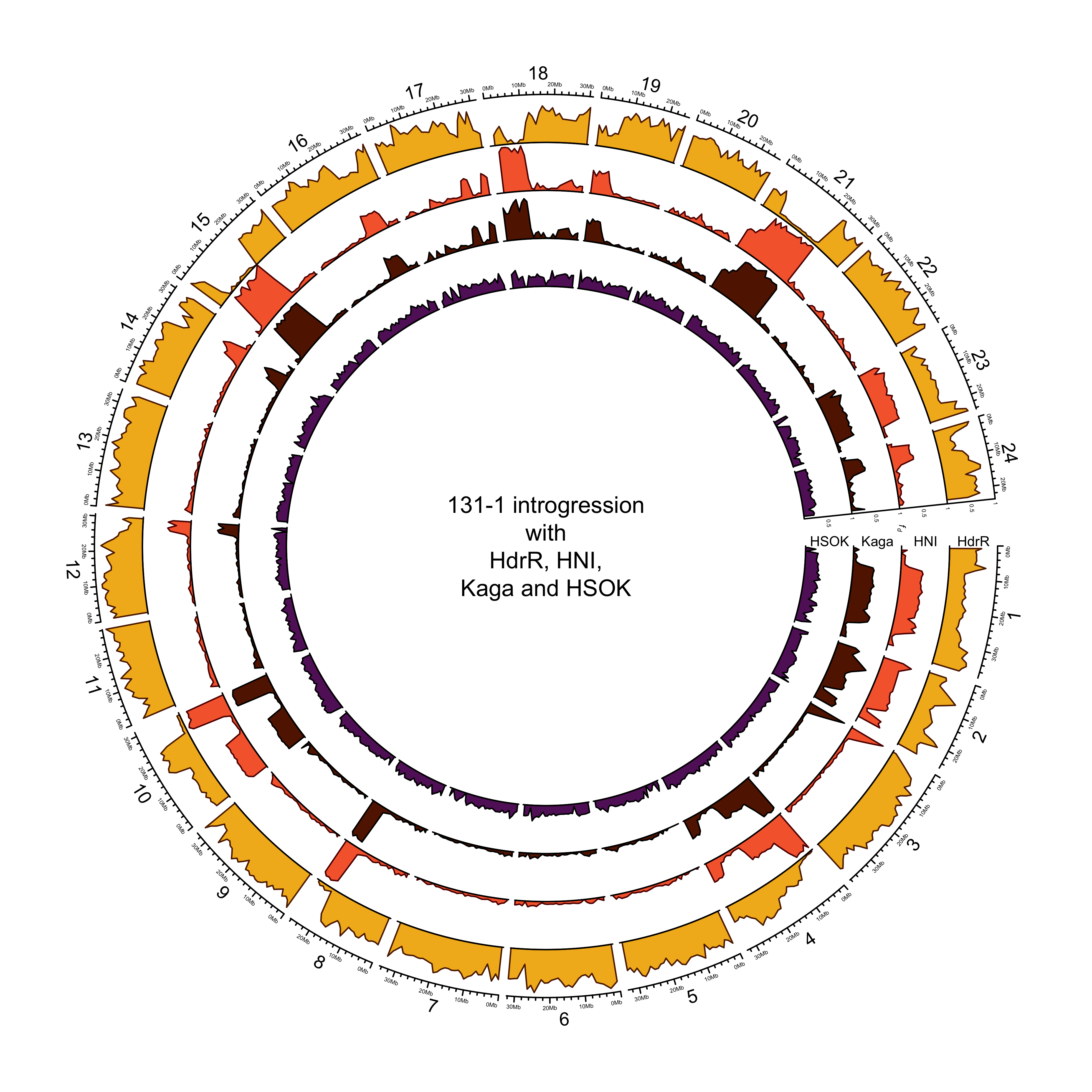
More introgression with HNI or Kaga?
intro_mikk$`131_1` %>%
  dplyr::bind_rows() %>%
  dplyr::filter(p2 %in% c("HNI", "Kaga")) %>%
  dplyr::group_by(p2) %>%
  dplyr::summarise(mean(mean_fd),
                   max(mean_fd))
## # A tibble: 2 × 3
##   p2    `mean(mean_fd)` `max(mean_fd)`
##   <fct>           <dbl>          <dbl>
## 1 HNI             0.198          0.986
## 2 Kaga            0.185          0.939
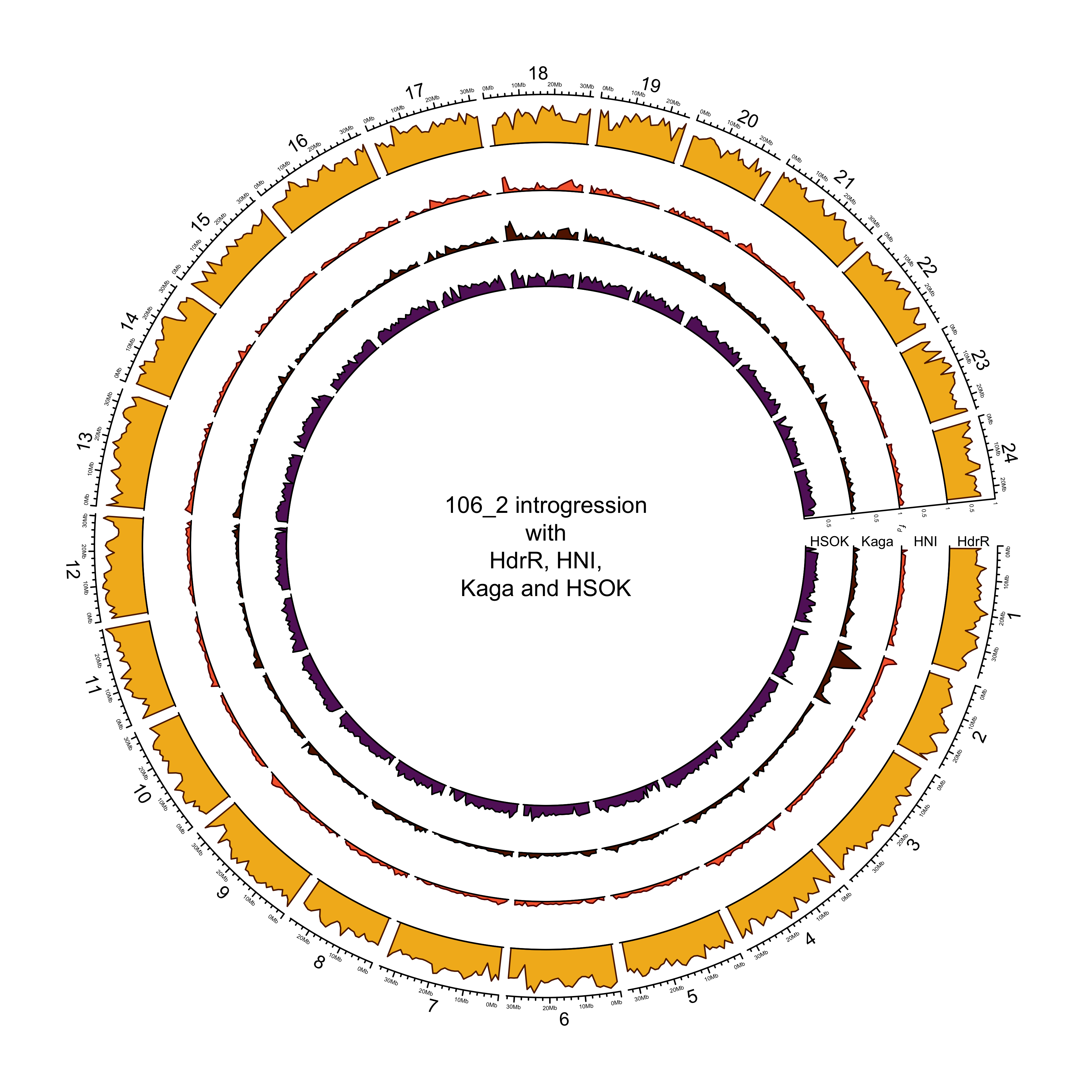
Do the same for each MIKK line
counter_mikk = 0
lapply(intro_mikk, function(MIKK_LINE){
  # Set counter_mikk
  counter_mikk <<- counter_mikk + 1
  # Set plot path
  out_plot = here::here("docs/plots/sv_analysis/20210330_circos_mikk",
                        paste(names(intro_mikk)[counter_mikk], ".png", sep = ""))
  # Generate plot
  png(out_plot,
      width = 20,
      height = 20,
      units = "cm",
      res = 500)

  # Set parameters
  ## Decrease cell padding from default c(0.02, 1.00, 0.02, 1.00)
  circos.par(cell.padding = c(0, 0, 0, 0),
             track.margin = c(0, 0),
             gap.degree = c(rep(1, nrow(chroms) - 1), 6))
  # Initialize plot
  circos.initializeWithIdeogram(chroms,
                                plotType = c("axis", "labels"),
                                major.by = 1e7,
                                axis.labels.cex = 0.25*par("cex"))

  # Print label in center
  text(0, 0, paste(names(intro_mikk)[counter_mikk],
                   " introgression\nwith\nHdrR, HNI,\nKaga and HSOK",
                   sep = ""))

  ###############
  # Introgression
  ###############
  counter = 0

  purrr::map(MIKK_LINE, function(P2){
    # Set counter
    counter <<- counter + 1

    circos.genomicTrack(P2,
        panel.fun = function(region, value, ...){
          circos.genomicLines(region,
                              value[[1]],
                              col = pal_abba[[names(MIKK_LINE[counter])]],
                              area = T,
                              border = karyoploteR::darker(pal_abba[[names(MIKK_LINE[counter])]]))
          # Add baseline
          circos.xaxis(h = "bottom",
                       labels = F,
                       major.tick = F)
        },
        track.height = 0.1,
        bg.border = NA,
        ylim = c(0, 1))

    # Add axis for introgression
    circos.yaxis(side = "right",
               at = c(.5, 1),
               labels.cex = 0.25*par("cex"),
               tick.length = 2
               )

    # Add y-axis label for introgression
    if (counter == 2) {
    circos.text(0, 0,
                labels = expression(italic(f[d])),
                sector.index = "chr1",
  #              facing = "clockwise",
                adj = c(3, 0.5),
                cex = 0.4*par("cex"))
    }

    # Add y-axis label for introgression
    circos.text(0, 0.5,
                labels = names(MIKK_LINE)[counter],
                sector.index = "chr1",
                facing = "clockwise",
                adj = c(.5, 0),
                cex = 0.6*par("cex"))
  })

  circos.clear()

  dev.off()
})
Example plot (all lines other than 131-1 look nearly identical).
knitr::include_graphics(here::here("docs/plots/sv_analysis/20210330_circos_mikk/106_2.png"))
Intersection with repeats
Read in HdrR repeats file
# Read in data
hdrr_reps = read.table(file.path(lts_dir, "repeats/medaka_hdrr_repeats.fixed.gff"),
                       header = F, sep = "\t", skip = 3, comment.char = "", quote = "", as.is = T) %>%
  # Remove empty V8 column
  dplyr::select(-V8) %>%
  # Get class of repeat from third column
  dplyr::mutate(class = stringr::str_split(V3, pattern = "#", simplify = T)[, 1]) %>%
  # Rename columns
  dplyr::rename(chr = V1, tool = V2, class_full = V3, start = V4, end = V5, percent = V6, strand = V7, info = V9)

# Find types of class other than "(GATCCA)n" types
class_types = unique(hdrr_reps$class[grep(")n", hdrr_reps$class, invert = T)])

hdrr_reps = hdrr_reps %>%
  # NA for blanks
  dplyr::mutate(class = dplyr::na_if(class, "")) %>%
  # "misc" for others in "(GATCCA)n" type classes
  dplyr::mutate(class = dplyr::if_else(!class %in% class_types, "Misc.", class)) %>%
  # rename "Simple_repeat"
  dplyr::mutate(class = dplyr::recode(class, "Simple_repeat" = "Simple repeat"))
Get total bases covered by each class of repeat
# Get ranges per class
hdrr_class_ranges = hdrr_reps %>%
  split(.$class) %>%
  purrr::map(., function(x){
    out = list()
    out[["RANGES"]] = GenomicRanges::makeGRangesFromDataFrame(x,
                                                              keep.extra.columns = T,
                                                              seqnames.field = "chr",
                                                              start.field = "start",
                                                              end.field = "end")
    out[["NON_OVERLAPPING"]] = disjoin(out[["RANGES"]])
    out[["COVERAGE_BY_CHR"]] = tibble(CHR = as.vector(seqnames(out[["NON_OVERLAPPING"]])),
                                      WIDTH = width(out[["NON_OVERLAPPING"]])) %>%
      dplyr::group_by(CHR) %>%
      dplyr::summarise(COVERED = sum(WIDTH)) %>%
      dplyr::ungroup() %>%
      dplyr::mutate(CHR = factor(CHR, levels = c(1:24, "MT"))) %>%
      dplyr::arrange(CHR)

    out[["TOTAL_COVERED"]] = sum(width(out[["NON_OVERLAPPING"]]))

    return(out)
  })

# Coverage per SVTYPE
repeat_cov_by_class = hdrr_class_ranges %>%
  purrr::map_int("TOTAL_COVERED") %>%
  tibble(CLASS = names(.),
         BASES_COVERED = .)

# Total percentage of genome covered by repeats (irrespective of strand)
total_repeat_cov = hdrr_reps %>%
  dplyr::select(-strand) %>%
  GenomicRanges::makeGRangesFromDataFrame(.,
                                          keep.extra.columns = T,
                                          ignore.strand = T,
                                          seqnames.field = "chr",
                                          start.field = "start",
                                          end.field = "end") %>%
  disjoin(.) %>%
  width(.) %>%
  sum(.)

total_repeat_cov / sum(chroms$end)
## [1] 0.1629319
# Get counts to tell frequency of occurrence

## First get total Mb in HdrR reference
hdrr_mb = sum(chroms$end) / 1e6

hdrr_rep_counts = hdrr_reps %>%
  dplyr::rename(CLASS = class) %>%
  dplyr::mutate(LENGTH = end - start) %>%
  group_by(CLASS) %>%
  summarise(N = n(),
            MEDIAN_LENGTH = median(LENGTH))
Find intersections with SVs
Get discrete ranges for HdrR repeats
# Convert to ranges
hdrr_reps_ranges = hdrr_reps %>%
  # remove strand column to avoid `names of metadata columns cannot be one of "seqnames", "ranges", "strand"...` error
  dplyr::select(-strand) %>%
  GenomicRanges::makeGRangesFromDataFrame(.,
                                          keep.extra.columns = T,
                                          ignore.strand = T,
                                          seqnames.field = "chr",
                                          start.field = "start",
                                          end.field = "end")

head(hdrr_reps_ranges)
## GRanges object with 6 ranges and 5 metadata columns:
##       seqnames    ranges strand |         tool         class_full   percent                   info       class
##          <Rle> <IRanges>  <Rle> |  <character>        <character> <numeric>            <character> <character>
##   [1]        1    54-131      * | RepeatMasker              DNA#P      14.5 Target "Motif:rnd-4_..         DNA
##   [2]        1    85-144      * | RepeatMasker            Unknown      16.7 Target "Motif:rnd-6_..     Unknown
##   [3]        1   789-866      * | RepeatMasker SINE#tRNA-Core-RTE      19.5 Target "Motif:rnd-6_..        SINE
##   [4]        1   921-947      * | RepeatMasker              (CA)n      12.2   Target "Motif:(CA)n"       Misc.
##   [5]        1 4464-4596      * | RepeatMasker            LINE#L2      26.9 Target "Motif:DF0004..        LINE
##   [6]        1 4478-4599      * | RepeatMasker            LINE#L2      28.7 Target "Motif:DF0003..        LINE
##   -------
##   seqinfo: 25 sequences from an unspecified genome; no seqlengths
# Number of bases covered by some sort of repeat
reduce(hdrr_reps_ranges) %>%
  width(.) %>%
  sum(.)
## [1] 119598609
# What proportion of total bases?
reduce(hdrr_reps_ranges) %>%
  width(.) %>%
  sum(.) / sum(chroms$end)
## [1] 0.1629319
So about [one sixth]{color = “red”} of the HdrR genome is composed of repeats.
Convert polished SV df to GRanges and find overlaps
sv_ranges_list = sv_df %>%
  dplyr::filter(DATASET == "polished") %>%
  # For all TRA, set STOP as POS
  dplyr::mutate(STOP = dplyr::if_else(SVTYPE == "TRA",
                                      POS,
                                      END)) %>%
  # For 9066/265857 INS and 272/23991 DUP where END is less than POS, set `STOP` as same as `POS`
  dplyr::mutate(STOP = dplyr::if_else(SVTYPE %in% c("INS", "DUP") & END < POS,
                                      POS,
                                      STOP)) %>%
  # Remove "chr" prefix" from CHROM
  dplyr::mutate(CHROM = str_remove(CHROM, "chr")) %>%
  # Split by SVTYPE
  split(.$SVTYPE) %>%
  # Loop over each SVTYPE
  purrr::map(., function(x) {
    out = list()
    # Keep original SV df
    out[["SV_df"]] = x
    # Convert to ranges
    out[["SV_Ranges"]] = GenomicRanges::makeGRangesFromDataFrame(x,
                                            keep.extra.columns = T,
                                            ignore.strand = T,
                                            seqnames.field = "CHROM",
                                            start.field = "POS",
                                            end.field = "STOP",
                                            strand.field = "ST")
    # Find overlaps with repeats
    out[["Overlaps"]] = findOverlaps(out[["SV_Ranges"]],
                                     hdrr_reps_ranges,
                                     ignore.strand = T)
    # Create DF with SV index and overlapping repeats
    SV_INDEX = queryHits(out[["Overlaps"]]) # Pull out all SV indices
    s_hits = hdrr_reps_ranges[subjectHits(out[["Overlaps"]])] # Pull out all repeat matches
    out[["Matches"]] = cbind(SV_INDEX, # Bind into data frame with SV index
                             REPEAT_LENGTH = width(s_hits), # Length of repeat
                             as.data.frame(mcols(s_hits))) # And repeat metadata
    return(out)
  })
Get stats on number and type of overlaps
sv_overlap_stats = lapply(sv_ranges_list, function(x){
  out = list()
  out[["TOTAL_SVS"]] = nrow(x[["SV_df"]])
  out[["TOTAL_OVERLAPPING_REPEAT"]] = length(unique(x[["Matches"]]$SV_INDEX))
  out[["PROP_OVERLAPPING"]] = out[["TOTAL_OVERLAPPING_REPEAT"]] / out[["TOTAL_SVS"]]
  out[["MEDIAN_MATCHES"]] = x[["Matches"]] %>% count(SV_INDEX) %>% summarise(median(n)) %>% pull
  out[["REPEAT_CLASS_COUNTS"]] = x[["Matches"]] %>% count(class)
  return(out)
})

# Get proportions of SVs with overlap
map_dbl(sv_overlap_stats, "PROP_OVERLAPPING")
##       DEL       DUP       INS       INV       TRA
## 0.7175866 0.6300279 0.2087852 0.8057308 0.3466956
How many DEL bases overlap with repeats?
# Total DEL bases
total_del_bases = GenomicRanges::reduce(sv_ranges_list$DEL$SV_Ranges)
total_del_bases = sum(BiocGenerics::width(total_del_bases))

total_del_bases
## [1] 111639227
# Total DEL bases intersecting with repeats
total_del_rep_ints = GenomicRanges::intersect(sv_ranges_list$DEL$SV_Ranges, hdrr_reps_ranges)
total_del_rep_ints = sum(BiocGenerics::width(total_del_rep_ints))

total_del_rep_ints
## [1] 34225753
# Percentage of DEL bases intersecting with repeats
total_del_rep_ints / total_del_bases
## [1] 0.3065746
Why so few overlaps for INS? Check INS length based on whether they overlap or not
sv_ranges_list$INS$SV_df %>%
  # Create index
  dplyr::mutate(SV_INDEX = rownames(.),
                # Get yes/no vector for whether they overlap repeats
                OVERLAPPING_REPEAT = dplyr::if_else(SV_INDEX %in% sv_ranges_list$INS$Matches$SV_INDEX,
                                                    "yes",
                                                    "no")) %>%
  ggplot(aes(OVERLAPPING_REPEAT, LN, colour = OVERLAPPING_REPEAT)) +
    geom_boxplot() +
    scale_y_log10() +
    theme_cowplot() +
    guides(colour = "none") +
    xlab("Overlapping repeat") +
    ylab("INS length")

ggsave(here::here("docs/plots/sv_analysis/20210409_INS_repeat_overlap.png"),
       device = "png",
       dpi = 400,
       units = "cm",
       width = 20,
       height = 12)
Intersection with pLI regions
pli_file = here::here("data/sv_analysis/unique_medaka_hgnc_link_with_pLI_and_annotations.txt")

# Read in data
pli_df = readr::read_tsv(pli_file,
                         trim_ws = T) %>%
  # remove rows with NA in chr
  dplyr::filter(!is.na(chr)) %>%
  # order
  dplyr::arrange(chr, start) %>%
  # remove strand column to avoid the following error when converting to GRanges:`names of metadata columns cannot be one of "seqnames", "ranges", "strand"`
  dplyr::select(-strand) %>%
  # create PLI_INDEX
  dplyr::mutate(PLI_INDEX = rownames(.))

# Convert to genomic ranges
pli_ranges = GenomicRanges::makeGRangesFromDataFrame(pli_df,
                                            keep.extra.columns = T,
                                            ignore.strand = T,
                                            seqnames.field = "chr",
                                            start.field = "start",
                                            end.field = "stop")

pli_ranges
## GRanges object with 12566 ranges and 12 metadata columns:
<<<<<<< HEAD
##           seqnames        ranges strand |            gene_id            gene_id.1   hgnc_id   gene_name         pLI n_gwas_hits          mapped_traits
##              <Rle>     <IRanges>  <Rle> |        <character>          <character> <numeric> <character>   <numeric>   <numeric>            <character>
##       [1]        1  92003-119620      * | ENSORLG00000019899 ENSORLG00000019899.2     11187        SOS1 9.99999e-01           3 Corticobasal degener..
##       [2]        1 153964-160887      * | ENSORLG00000018405 ENSORLG00000018405.2     18683      EIF4A3 9.98064e-01          15 response to antineop..
##       [3]        1 232322-247327      * | ENSORLG00000020897 ENSORLG00000020897.2     21022       AARS2 2.52762e-05           1 interleukin 10 measu..
##       [4]        1 333629-337606      * | ENSORLG00000019696 ENSORLG00000019696.2     26643        SDE2 1.00544e-05           1 attention deficit hy..
##       [5]        1 438626-448849      * | ENSORLG00000020895 ENSORLG00000020895.2     15858      DZANK1 4.95681e-13           0                   <NA>
##       ...      ...           ...    ... .                ...                  ...       ...         ...         ...         ...                    ...
##   [12562]       MT   10044-10340      * | ENSORLG00000021774 ENSORLG00000021774.1      7460     MT-ND4L          NA           0                   <NA>
##   [12563]       MT   10334-11714      * | ENSORLG00000021775 ENSORLG00000021775.1      7459      MT-ND4          NA           0                   <NA>
##   [12564]       MT   11932-13770      * | ENSORLG00000021779 ENSORLG00000021779.1      7461      MT-ND5          NA           0                   <NA>
##   [12565]       MT   13766-14287      * | ENSORLG00000021780 ENSORLG00000021780.1      7462      MT-ND6          NA           0                   <NA>
##   [12566]       MT   14359-15499      * | ENSORLG00000021782 ENSORLG00000021782.1      7427      MT-CYB          NA           0                   <NA>
##                           p_vals             accessions                   snps                context   PLI_INDEX
##                      <character>            <character>            <character>            <character> <character>
##       [1] 6.69897000433602|5.5.. GCST002971|GCST00297.. rs963731|rs963731|rs.. intron_variant|intro..           1
##       [2] 5.09691001300806|5.2.. GCST001692|GCST00176.. rs12954803|rs7235440.. intergenic_variant|i..           2
##       [3]       5.52287874528034             GCST004444            rs201200147         intron_variant           3
##       [4]       5.22184874961636             GCST003473             rs12737863     intergenic_variant           4
##       [5]                   <NA>                   <NA>                   <NA>                   <NA>           5
##       ...                    ...                    ...                    ...                    ...         ...
##   [12562]                   <NA>                   <NA>                   <NA>                   <NA>       12562
##   [12563]                   <NA>                   <NA>                   <NA>                   <NA>       12563
##   [12564]                   <NA>                   <NA>                   <NA>                   <NA>       12564
##   [12565]                   <NA>                   <NA>                   <NA>                   <NA>       12565
##   [12566]                   <NA>                   <NA>                   <NA>                   <NA>       12566
=======
##           seqnames        ranges strand |            gene_id            gene_id.1   hgnc_id   gene_name         pLI
##              <Rle>     <IRanges>  <Rle> |        <character>          <character> <numeric> <character>   <numeric>
##       [1]        1  92003-119620      * | ENSORLG00000019899 ENSORLG00000019899.2     11187        SOS1 9.99999e-01
##       [2]        1 153964-160887      * | ENSORLG00000018405 ENSORLG00000018405.2     18683      EIF4A3 9.98064e-01
##       [3]        1 232322-247327      * | ENSORLG00000020897 ENSORLG00000020897.2     21022       AARS2 2.52762e-05
##       [4]        1 333629-337606      * | ENSORLG00000019696 ENSORLG00000019696.2     26643        SDE2 1.00544e-05
##       [5]        1 438626-448849      * | ENSORLG00000020895 ENSORLG00000020895.2     15858      DZANK1 4.95681e-13
##       ...      ...           ...    ... .                ...                  ...       ...         ...         ...
##   [12562]       MT   10044-10340      * | ENSORLG00000021774 ENSORLG00000021774.1      7460     MT-ND4L          NA
##   [12563]       MT   10334-11714      * | ENSORLG00000021775 ENSORLG00000021775.1      7459      MT-ND4          NA
##   [12564]       MT   11932-13770      * | ENSORLG00000021779 ENSORLG00000021779.1      7461      MT-ND5          NA
##   [12565]       MT   13766-14287      * | ENSORLG00000021780 ENSORLG00000021780.1      7462      MT-ND6          NA
##   [12566]       MT   14359-15499      * | ENSORLG00000021782 ENSORLG00000021782.1      7427      MT-CYB          NA
##           n_gwas_hits          mapped_traits                 p_vals             accessions                   snps
##             <numeric>            <character>            <character>            <character>            <character>
##       [1]           3 Corticobasal degener.. 6.69897000433602|5.5.. GCST002971|GCST00297.. rs963731|rs963731|rs..
##       [2]          15 response to antineop.. 5.09691001300806|5.2.. GCST001692|GCST00176.. rs12954803|rs7235440..
##       [3]           1 interleukin 10 measu..       5.52287874528034             GCST004444            rs201200147
##       [4]           1 attention deficit hy..       5.22184874961636             GCST003473             rs12737863
##       [5]           0                   <NA>                   <NA>                   <NA>                   <NA>
##       ...         ...                    ...                    ...                    ...                    ...
##   [12562]           0                   <NA>                   <NA>                   <NA>                   <NA>
##   [12563]           0                   <NA>                   <NA>                   <NA>                   <NA>
##   [12564]           0                   <NA>                   <NA>                   <NA>                   <NA>
##   [12565]           0                   <NA>                   <NA>                   <NA>                   <NA>
##   [12566]           0                   <NA>                   <NA>                   <NA>                   <NA>
##                          context   PLI_INDEX
##                      <character> <character>
##       [1] intron_variant|intro..           1
##       [2] intergenic_variant|i..           2
##       [3]         intron_variant           3
##       [4]     intergenic_variant           4
##       [5]                   <NA>           5
##       ...                    ...         ...
##   [12562]                   <NA>       12562
##   [12563]                   <NA>       12563
##   [12564]                   <NA>       12564
##   [12565]                   <NA>       12565
##   [12566]                   <NA>       12566
>>>>>>> 1f72b2c38317bbf9e22e15671a199f851eaded2e
##   -------
##   seqinfo: 25 sequences from an unspecified genome; no seqlengths
Get overlaps
pli_overlaps = purrr::map(sv_ranges_list, function(SVTYPE){

  out = list()

  # Find overlaps with repeats
  out[["Overlaps"]] = findOverlaps(SVTYPE[["SV_Ranges"]],
                                   pli_ranges,
                                   ignore.strand = T)

  # Create DF with SV index and overlapping repeats
  SV_INDEX = queryHits(out[["Overlaps"]]) # Pull out all SV indices
  s_hits = pli_ranges[subjectHits(out[["Overlaps"]])] # Pull out all repeat matches
  out[["Matches"]] = cbind(SV_INDEX, # Bind into data frame with SV index
                           REPEAT_LENGTH = width(s_hits), # Length of gene
                           as.data.frame(mcols(s_hits))) # And gene metadata

  return(out)
})
Split by SV and calculate LOD for each
lod_list = purrr::map(pli_overlaps, function(SVTYPE){
  SVTYPE[["Matches"]] %>%
    split(f = .$SV_INDEX) %>%
      purrr::map(., function(SV){
        # Create list of matching PLI_INDEXes
        pli_inds = list(SV$PLI_INDEX)
        # Summarise other columns
        SV %>%
          dplyr::summarise(N_OVERLAPPING_GENES = n(),
                           LOD = LOD(pLI),
                           PLI_INDEX_MATCHES = I(pli_inds))
      }) %>%
    dplyr::bind_rows(.id = "SV_INDEX") %>%
    dplyr::mutate(SV_INDEX = as.integer(SV_INDEX))
})
Bind with original SV df
sv_lod = purrr::map(type_order, function(SVTYPE){

  out = sv_ranges_list[[SVTYPE]][["SV_df"]] %>%
    # create DF with SV_INDEX for binding
    dplyr::mutate(SV_INDEX = as.integer(rownames(.))) %>%
    # bind LOD score
    dplyr::left_join(lod_list[[SVTYPE]],
                     by = "SV_INDEX")

  return(out)
})

names(sv_lod) = type_order

# Bind into single DF
sv_lod_df = sv_lod %>%
  dplyr::bind_rows()

# Take only distinct SVs
sv_lod_df = sv_lod_df %>%
  dplyr::filter(!duplicated(ID)) %>%
  dplyr::select(-SAMPLE)
LOD score by SV LN and SVTYPE
How many SVs overlap genes?
sv_lod_df %>%
  dplyr::filter(SVTYPE != "TRA") %>%
  summarise(TOTAL = n(),
            # count number of SVs with at least one overlapping gene
            N_OVERLAPPING = sum(!is.na(N_OVERLAPPING_GENES)),
            PROP_N_OVERLAPPING = N_OVERLAPPING/TOTAL,
            MAX = max(N_OVERLAPPING_GENES, na.rm = T))
## # A tibble: 1 × 4
##    TOTAL N_OVERLAPPING PROP_N_OVERLAPPING   MAX
##    <int>         <int>              <dbl> <int>
## 1 134088         33146              0.247    91
Histogram of number of overlapping genes
sv_lod_df %>%
  dplyr::filter(SVTYPE != "TRA",
                !is.na(N_OVERLAPPING_GENES)) %>%
  dplyr::mutate(SVTYPE = factor(SVTYPE, levels = names(svtype_hist_pal))) %>%
  ggplot() +
    geom_histogram(aes(N_OVERLAPPING_GENES, fill = SVTYPE)) +
    scale_fill_manual(values = svtype_hist_pal) +
    theme_bw() +
    scale_x_log10()
## `stat_bin()` using `bins = 30`. Pick better value with `binwidth`.

Filter out TRA and NAs
sv_lod_plot_df = sv_lod_df %>%
  dplyr::filter(SVTYPE != "TRA",
                !is.na(LOD)) %>%
  dplyr::mutate(SVTYPE = factor(SVTYPE, levels = names(svtype_hist_pal)))
Plot
sv_lod_plot = sv_lod_plot_df %>%
  ggplot(aes(log10(LN), LOD)) +
    geom_point(aes(colour = SVTYPE), size = 1, alpha = .1) +
    facet_wrap(~SVTYPE, nrow = 2, ncol = 2) +
    scale_colour_manual(values = svtype_hist_pal) +
    theme_cowplot() +
    guides(colour = "none") +
    xlab(expression(log[10](length))) +
    ylab("LOD for pLI") +
    theme(axis.text.x = element_text(size = 6),
          strip.text = element_text(face = "bold"),
          strip.background = element_blank()
          )

sv_lod_plot = sv_lod_plot +
  geom_smooth(data = sv_lod_plot_df %>% dplyr::filter(SVTYPE == "DEL"),
             aes(log10(LN), LOD), colour = darker(svtype_hist_pal[["DEL"]], amount = 100)) +
  geom_smooth(data = sv_lod_plot_df %>% dplyr::filter(SVTYPE == "INS"),
             aes(log10(LN), LOD), colour = darker(svtype_hist_pal[["INS"]], amount = 100)) +
  geom_smooth(data = sv_lod_plot_df %>% dplyr::filter(SVTYPE == "DUP"),
             aes(log10(LN), LOD), colour = darker(svtype_hist_pal[["DUP"]], amount = 100)) +
  geom_smooth(data = sv_lod_plot_df %>% dplyr::filter(SVTYPE == "INV"),
             aes(log10(LN), LOD), colour = darker(svtype_hist_pal[["INV"]], amount = 100))

sv_lod_plot
## `geom_smooth()` using method = 'gam' and formula 'y ~ s(x, bs = "cs")'
## Warning: Removed 5 rows containing non-finite values (stat_smooth).
## `geom_smooth()` using method = 'gam' and formula 'y ~ s(x, bs = "cs")'
## Warning: Removed 4 rows containing non-finite values (stat_smooth).
## `geom_smooth()` using method = 'gam' and formula 'y ~ s(x, bs = "cs")'
## Warning: Removed 1 rows containing non-finite values (stat_smooth).
## `geom_smooth()` using method = 'loess' and formula 'y ~ x'

ggsave(here::here("docs/plots/sv_analysis/20210407_pli_lod.png"),
       device = "png",
       width = 30,
       height = 20,
       units = "cm",
       dpi = 400)
Histogram of LOD
sv_lod_hist = sv_lod_plot_df %>%
  ggplot() +
#    geom_density(aes(LOD, fill = SVTYPE), position = "stack") +
    geom_histogram(aes(LOD, fill = SVTYPE), bins = 70) +
    scale_fill_manual(values = svtype_hist_pal) +
    theme_cowplot() +
    guides(fill = "none") +
    scale_y_log10() +
    ylab(expression(log[10](count))) +
    xlab("LOD for pLI")

sv_lod_hist
## Warning: Removed 10 rows containing non-finite values (stat_bin).
## Warning: Transformation introduced infinite values in continuous y-axis
## Warning: Removed 121 rows containing missing values (geom_bar).

Stats for paper
How many SVs overlapped at least one gene
unique_svs = length(unique(sv_df_pol %>%
                             dplyr::filter(SVTYPE != "TRA") %>%
                             dplyr::pull(ID)))

overlapping_svs = sv_lod_plot_df %>%
  dplyr::pull(ID) %>%
  unique(.) %>%
  length(.)

unique_svs
## [1] 134088
## [1] 30357
overlapping_svs / unique_svs
## [1] 0.2263961
How many SVs with LOD > 0?
sv_lod_plot_df %>%
  summarise(TOTAL = n(),
            N_OVER_0 = sum(LOD > 0),
            N_OVER_10 = sum(LOD > 10),
            PROP_OVER_0 = N_OVER_0 / TOTAL,
            PROP_OVER_10 = N_OVER_10 / TOTAL,
            LOD_90_PERC = quantile(LOD, 0.9))
## # A tibble: 1 × 6
##   TOTAL N_OVER_0 N_OVER_10 PROP_OVER_0 PROP_OVER_10 LOD_90_PERC
##   <int>    <int>     <int>       <dbl>        <dbl>       <dbl>
## 1 30357    16111      2588       0.531       0.0853        9.05
Pull out high-LOD regions
sv_lod_df %>%
  dplyr::filter(LOD > 50)
## # A tibble: 2 × 18
<<<<<<< HEAD
##   DATASET  CHROM      POS    ID ALT   FILTER SVLEN SVTYPE CHR2       END GT       LN ST        STOP SV_INDEX N_OVERLAPPING_GENES   LOD PLI_INDEX_MATCH…
##   <fct>    <chr>    <int> <int> <chr> <chr>  <int> <chr>  <chr>    <int> <chr> <int> <chr>    <int>    <int>               <int> <dbl> <I<list>>
## 1 polished 2     15933747 20346 <INS> PASS     243 INS    2     15933747 0/1     236 +-    15933747   122844                   5  53.7 <chr [5]>
## 2 polished 2     15922253 20343 <INS> PASS    1127 INS    2     15922253 0/1    1097 +-    15922253   238864                   5  53.7 <chr [5]>
=======
## DATASET CHROM POS ID ALT FILTER SVLEN SVTYPE CHR2 END GT LN ST STOP SV_INDEX N_OVERLAPPING_G…
## <fct> <chr> <int> <int> <chr> <chr> <int> <chr> <chr> <int> <chr> <int> <chr> <int> <int> <int>
## 1 polished 2 15933747 20346 <INS> PASS 243 INS 2 15933747 0/1 236 +- 15933747 122844 5
## 2 polished 2 15922253 20343 <INS> PASS 1127 INS 2 15922253 0/1 1097 +- 15922253 238864 5
## # … with 2 more variables: LOD <dbl>, PLI_INDEX_MATCHES <I<list>>
>>>>>>> 1f72b2c38317bbf9e22e15671a199f851eaded2e
# Get indexes of overlapping genes
sv_lod_df %>%
  dplyr::filter(LOD > 50) %>%
  dplyr::group_by(SV_INDEX) %>%
  dplyr::pull(PLI_INDEX_MATCHES)
[[1]] [1] “786” “787” “788” “789” “790”
[[2]] [1] “786” “787” “788” “789” “790”
# All the same. Take all
high_lod = sv_lod_df %>%
  dplyr::filter(LOD > 50) %>%
  dplyr::group_by(SV_INDEX) %>%
  dplyr::pull(PLI_INDEX_MATCHES) %>%
  unlist(.) %>%
  unique(.)

# Get pLI matches
DT::datatable(pli_df[high_lod, ])
<<<<<<< HEAD
=======
>>>>>>> 1f72b2c38317bbf9e22e15671a199f851eaded2e
New final figure
final_svtype = ggdraw() +
  draw_image(here::here("docs/plots/sv_analysis/20210325_sv_dels_lines.png"),
           x = 0, y = 0, width = 1, height = .6, scale = 1.12) +
  draw_plot(svlen_counts_plot,
            x = 0, y = .8, width =.4, height = .2) +
  draw_plot(sv_lod_plot,
            x = .4, y = .8, width =.6, height = .2) +
  draw_plot(sv_lod_hist,
            x = 0, y = .6, width = .4, height = .2) +
  draw_plot(svtype_counts_plot,
            x = .4, y = .6, width = .6, height = .2) +
  draw_plot_label(label = c("A", "B", "C", "D", "E"),
                  x = c(0, .4, 0, .4, 0),
                  y = c(1, 1, .8, .8, .6),
                  size = 25,color = "#4f0943")
## `geom_smooth()` using method = 'gam' and formula 'y ~ s(x, bs = "cs")'
## Warning: Removed 5 rows containing non-finite values (stat_smooth).
## `geom_smooth()` using method = 'gam' and formula 'y ~ s(x, bs = "cs")'
## Warning: Removed 4 rows containing non-finite values (stat_smooth).
## `geom_smooth()` using method = 'gam' and formula 'y ~ s(x, bs = "cs")'
## Warning: Removed 1 rows containing non-finite values (stat_smooth).
## `geom_smooth()` using method = 'loess' and formula 'y ~ x'
## Warning: Removed 10 rows containing non-finite values (stat_bin).
## Warning: Transformation introduced infinite values in continuous y-axis
## Warning: Removed 121 rows containing missing values (geom_bar).

ggsave(here::here("docs/plots/sv_analysis/20210325_sv_dels_lines.png"),
       device = "png",
       dpi = 400,
       units = "cm",
       width = 30,
       height = 42)
Find overlaps with genes and exons
Get ranges
Genes and exons
# Get list of genes and exons from biomaRt

## Select dataset
olat_mart = biomaRt::useEnsembl(biomart = "ensembl", dataset = "olatipes_gene_ensembl")

## Convert genes to GRanges
gene_ranges = biomaRt::getBM(attributes = c("chromosome_name",
                                            "start_position",
                                            "end_position",
                                            "ensembl_gene_id"),
                             mart = olat_mart) %>%
  GenomicRanges::makeGRangesFromDataFrame(ignore.strand = T,
                                          seqnames.field = "chromosome_name",
                                          start.field = "start_position",
                                          end.field = "end_position")
## Convert exons to GRanges
exon_ranges = biomaRt::getBM(attributes = c("chromosome_name",
                                            "exon_chrom_start",
                                            "exon_chrom_end",
                                            "ensembl_gene_id",
                                            "ensembl_transcript_id",
                                            "ensembl_exon_id"),
                             mart = olat_mart) %>%
  GenomicRanges::makeGRangesFromDataFrame(ignore.strand = T,
                                          seqnames.field = "chromosome_name",
                                          start.field = "exon_chrom_start",
                                          end.field = "exon_chrom_end")
Stats on ranges
# Number of ranges
## Genes
length(gene_ranges)
## [1] 24365
## Exons
length(exon_ranges)
## [1] 404636
# Total bases covered by
## Genes
gene_bases = gene_ranges %>%
  disjoin(.) %>%
  width(.) %>%
  sum(.)
## Exons
exon_bases = exon_ranges %>%
  disjoin(.) %>%
  width(.) %>%
  sum(.)

# Percentage bases covered
## Genes
gene_bases / sum(chroms$end) * 100
## [1] 55.16376
## Exons
exon_bases / sum(chroms$end) * 100
## [1] 9.385916
SVs
sv_ranges_novel = sv_df_pol %>%
  dplyr::filter(!duplicated(ID)) %>%
  # For all TRA, set STOP as POS
  dplyr::mutate(STOP = dplyr::if_else(SVTYPE == "TRA",
                                      POS,
                                      END)) %>%
  # For 9066/265857 INS and 272/23991 DUP where END is less than POS, set `STOP` as same as `POS`
  dplyr::mutate(STOP = dplyr::if_else(SVTYPE %in% c("INS", "DUP") & END < POS,
                                      POS,
                                      STOP)) %>%
  # Remove "chr" prefix" from CHROM
  dplyr::mutate(CHROM = str_remove(CHROM, "chr")) %>%
  # Conver to ranges
  GenomicRanges::makeGRangesFromDataFrame(ignore.strand = T,
                                          seqnames.field = "CHROM",
                                          start.field = "POS",
                                          end.field = "STOP")
Find overlaps
# With genes
gene_olaps = findOverlaps(sv_ranges_novel,
                          gene_ranges,
                          ignore.strand = T)

# With exons
exon_olaps = findOverlaps(sv_ranges_novel,
                          exon_ranges,
                          ignore.strand = T)


# Total SVs
length(sv_ranges_novel)
## [1] 143326
# How many SVs overlap genes
length(unique(queryHits(gene_olaps)))
## [1] 74271
# How many SVs overlap exons
length(unique(queryHits(exon_olaps)))
## [1] 11448
Find overlaps between DEL and INS based on reference-anchored and graph genome approaches
Read in data
High-confidence graph calls
googledrive::drive_get("MIKK SV assemblies paper",
                       shared_drive = googledrive::shared_drive_get("Indigene")) %>%
  googledrive::drive_ls(.)
## ℹ Suitable tokens found in the cache, associated with these emails:
## • 'brettell@ebi.ac.uk'
## • 'ian.brettell@googlemail.com'
## Defaulting to the first email.
## ! Using an auto-discovered, cached token.
## To suppress this message, modify your code or options to clearly consent to the use of a cached token.
## See gargle's "Non-interactive auth" vignette for more details:
## <https://gargle.r-lib.org/articles/non-interactive-auth.html>
## ℹ The googledrive package is using a cached token for 'brettell@ebi.ac.uk'.
## Auto-refreshing stale OAuth token.
## ✓ The input `path` resolved to exactly 1 file.
## # A dribble: 4 × 3
##   name                                                    id                                           drive_resource
##   <chr>                                                   <drv_id>                                     <list>
## 1 GB_revisions                                            1z3w4cVemfLgy3rqjkyedZMm9dzySFSBY            <named list [31]>
<<<<<<< HEAD
## 2 Figures and tables                                      1jxseUwEzJso34T4gqanJFqI2XoM6yqGP            <named list [31]>
## 3 The Inbred Medaka Kiyosu (MIKK) Panel SV and assemblies 1CWsa3LIsj2eIUq0mGbeb79encxXK34HawE3xq_jYGhs <named list [33]>
=======
## 2 The Inbred Medaka Kiyosu (MIKK) Panel SV and assemblies 1CWsa3LIsj2eIUq0mGbeb79encxXK34HawE3xq_jYGhs <named list [33]>
## 3 Figures and tables                                      1jxseUwEzJso34T4gqanJFqI2XoM6yqGP            <named list [31]>
>>>>>>> 1f72b2c38317bbf9e22e15671a199f851eaded2e
## 4 Genome Biology Submission                               1byuYSYf7CnndJ5FX9psjEsDbFDJ4jEAJ            <named list [32]>
tables_id = googledrive::drive_ls(googledrive::as_id("1jxseUwEzJso34T4gqanJFqI2XoM6yqGP"))
tables_id
## # A dribble: 14 × 3
##    name                                    id                                           drive_resource
##    <chr>                                   <drv_id>                                     <list>
##  1 graph_deletions_loci                    1-TGNnM1zHyclstVlFEtDSrmoeLCd53ZxAwNK5rO3SQw <named list [33]>
##  2 graph_alternative_divergent loci        1OMaJ25qAeDmLYv85h87ax26Q3RujGX7cTbViHzmESmg <named list [33]>
##  3 Supplementary figures                   1btIbLF-nwK8HUnc8hBeJqaw7ea5I-l0M            <named list [31]>
##  4 pycoMeth_summary_intervals              12yqF3CkX5K4ozC9IkPuFnAj48td55TSClTPsknY6d-8 <named list [32]>
##  5 Assembly_stats                          1mGdOXOmgHvhFF5ezJsTUX1gBCHC9n0VQf1VMkWfraGs <named list [32]>
##  6 Main figures                            1H3Y91wjBvZPfvdLV2TTmVzIx3gd4RWBf            <named list [31]>
##  7 Supplementary Tables                    1H9zxeVCU7RtRhNNa1_ZfFZ-2K6mI0aQO3DBJ6s3lfxM <named list [33]>
##  8 Supplementary Figures                   15_JG8k9i9_OOQDm9mZnKlasczaYHxdh-71w6C1qgsg4 <named list [33]>
##  9 Supplementary File 2 - Circos plots.pdf 1ejgyVKWCR-IC2UfeciuerFINgMiUs7yW            <named list [38]>
## 10 Supplementary File 1 - Karyoplots.pdf   1g8L3TawY1X1N2D2M6Mv1Qb6stNzigv4x            <named list [39]>
## 11 Segments Usage sample stats             1iiQNjVXPJSudoxLMoo8hnXUBbs63-pDbblkMd8tV2d0 <named list [32]>
## 12 Graph stats                             19svaqk0wJD-wp1vYiqlKBX45PR3WutPDiZeoLfqIJug <named list [32]>
## 13 Sequencing_stats                        1OyNh_HErz6Nl2EjI3-75yYkY5RObIznpn1daaHSmG9Q <named list [32]>
## 14 DNA_methylation                         1gD7CFExDIW8SV7Dve-a3IutW-Vz8xzQyHzlJSDv2IkM <named list [31]>
del_id = tables_id$id[tables_id$name == "graph_deletions_loci"]
ins_id = tables_id$id[tables_id$name == "graph_alternative_divergent loci"]
DEL
del_tbl = googlesheets4::read_sheet(del_id,
                                    range = "A1:A17") %>%
  tidyr::separate("HdrR locus", into = c("CHROM", "POS"), sep = ":", remove = F) %>%
  tidyr::separate("POS", into = c("START", "END"), sep = "-") %>%
  # convert to integer
  dplyr::mutate(dplyr::across(c("CHROM", "START", "END"),
                              ~as.integer(.x))) %>%
  dplyr::arrange(CHROM, START)
## ! Using an auto-discovered, cached token.
## To suppress this message, modify your code or options to clearly consent to the use of a cached token.
## See gargle's "Non-interactive auth" vignette for more details:
## <https://gargle.r-lib.org/articles/non-interactive-auth.html>
## ℹ The googlesheets4 package is using a cached token for 'brettell@ebi.ac.uk'.
## Auto-refreshing stale OAuth token.
## ✓ Reading from "graph_deletions_loci".
## ✓ Range 'A1:A17'.
INS
ins_tbl = googlesheets4::read_sheet(ins_id,
                                    range = "A1:A20") %>%
  # Remove the "HDRR_" prefix in the first row
  dplyr::mutate(`HdrR locus` = stringr::str_remove(`HdrR locus`, "HDRR_")) %>%
  tidyr::separate("HdrR locus", into = c("CHROM", "POS"), sep = ":", remove = F) %>%
  tidyr::separate("POS", into = c("START", "END"), sep = "-") %>%
  # convert to integer
  dplyr::mutate(dplyr::across(c("CHROM", "START", "END"),
                              ~as.integer(.x))) %>%
  dplyr::arrange(CHROM, START)
## ✓ Reading from "graph_alternative_divergent loci".
## ✓ Range 'A1:A20'.
Polished calls
pol_loci_file = file.path(lts_dir, "sv_analysis/loci/all.csv")
lines = c("4-1","7-1","11-1","69-1","79-2","80-1","117-2","131-1","134-1","134-2")
col_names = c("CHROM", "START", "END", "SVTYPE", "SVLEN", lines)

# Read in loci
polished_loci = readr::read_csv(pol_loci_file,
                                col_names = col_names,
                                col_types = c("cddcdcccccccccc")) %>%
  # remove MT
  dplyr::filter(CHROM != "MT") %>%
  # covert `CHROM` to integer
  dplyr::mutate(CHROM = as.integer(CHROM)) %>%
  # arrange by CHROM, POS
  dplyr::arrange(CHROM, START)

polished_loci_nomiss = polished_loci %>%
  # remove variants where all samples are missing
  dplyr::filter(dplyr::if_any(.cols = dplyr::all_of(lines),
                              .fns =  ~.x != "./.")) %>%
  # keep only variants where at least one sample has the alt allele
  dplyr::filter(dplyr::if_any(.cols = dplyr::all_of(lines),
                              .fns =  ~.x %in% c("0/1", "1/1"))) %>%
  # remove duplicated rows
  dplyr::distinct()

pol_loci_list = polished_loci_nomiss %>%
  # split into list by SVTYPE
  split(., f = .$SVTYPE)
Find overlaps
DEL
# Convert graph loci to GRanges
del_tbl_r = del_tbl %>%
  GenomicRanges::makeGRangesFromDataFrame(., ignore.strand = T)

# Convert polished loci to GRanges
del_pol_r = pol_loci_list$DEL %>%
  GenomicRanges::makeGRangesFromDataFrame(., ignore.strand = T, keep.extra.columns = T)

# Find overlaps
del_overlaps = IRanges::findOverlaps(del_tbl_r, del_pol_r)
del_overlaps
## Hits object with 66 hits and 0 metadata columns:
##        queryHits subjectHits
##        <integer>   <integer>
##    [1]         2       25618
##    [2]         2       25619
##    [3]         2       25620
##    [4]         2       25621
##    [5]         3       38017
##    ...       ...         ...
##   [62]        13       80893
##   [63]        15       82227
##   [64]        15       82228
##   [65]        15       82229
##   [66]        15       82230
##   -------
##   queryLength: 16 / subjectLength: 101863
# Get paired intersections
del_intersects = IRanges::pintersect(del_tbl_r[del_overlaps@from], del_pol_r[del_overlaps@to])
del_intersects
## GRanges object with 66 ranges and 1 metadata column:
##        seqnames            ranges strand |       hit
##           <Rle>         <IRanges>  <Rle> | <logical>
##    [1]        6   4103589-4114645      * |      TRUE
##    [2]        6   4103589-4114703      * |      TRUE
##    [3]        6   4103589-4114897      * |      TRUE
##    [4]        6   4106016-4108020      * |      TRUE
##    [5]        9   9672926-9673070      * |      TRUE
##    ...      ...               ...    ... .       ...
##   [62]       19   7041534-7051052      * |      TRUE
##   [63]       19 21994732-22004171      * |      TRUE
##   [64]       19 21994735-22004171      * |      TRUE
##   [65]       19 21998075-21998867      * |      TRUE
##   [66]       19 22003035-22003094      * |      TRUE
##   -------
##   seqinfo: 11 sequences from an unspecified genome; no seqlengths
<<<<<<< HEAD
# Create final data frame
del_final = tibble::tibble(# Graph deletion ranges and widths
                           del_tbl[del_overlaps@from, ] %>%
                             dplyr::rename(CHROM_G = CHROM,
                                           START_G = START,
                                           END_G = END),
                           WIDTH_G= BiocGenerics::width(del_tbl_r[del_overlaps@from, ]),
                           # Polished hits ranges and widths
                           del_pol_r[del_overlaps@to] %>%
                             GenomicRanges::granges(.) %>%
                             data.frame(.) %>%
                             dplyr::select(CHROM_P = seqnames,
                                           START_P = start,
                                           END_P = end,
                                           WIDTH_P = width),
                           # Add paired intersections
                           del_intersects %>%
                             GenomicRanges::granges(.) %>%
                             data.frame(.) %>%
                             dplyr::select(CHROM_I = seqnames,
                                           START_I = start,
                                           END_I = end,
                                           WIDTH_I = width),
                           # Add genotypes
                           pol_loci_list$DEL[del_overlaps@to, ] %>%
                             dplyr::select(all_of(lines))
                           ) %>%
  # Get proportion of graph variants covered by intersecting polished variants
  dplyr::mutate(PROP_COV = WIDTH_I / WIDTH_G)

DT::datatable(del_final)
# Find the maximum covered
del_max = del_final %>%
  dplyr::group_by(`HdrR locus`) %>%
  dplyr::slice_max(WIDTH_I) %>%
  # add SVs that had no overlaps and remove duplicates
  rbind(., del_tbl %>%
          dplyr::select(`HdrR locus`,
                        CHROM_G = CHROM,
                        START_G = START,
                        END_G = END) %>%
          dplyr::mutate(WIDTH_G = END_G - START_G + 1)) %>%
  dplyr::distinct(`HdrR locus`, .keep_all = T) %>%
  # Sort by chromosome and start position
  dplyr::arrange(CHROM_G, START_G) %>%
  # remove ties for WIDTH_I
  dplyr::distinct(`HdrR locus`, .keep_all = T) %>%
  # Unite polished locus
  tidyr::unite(col = POL_LOC, START_P, END_P, sep = "-") %>%
  tidyr::unite(col = `HdrR locus (reference-anchored)`, CHROM_P, POL_LOC, sep = ":") %>%
  # Unite intersection locus
  tidyr::unite(col = INT_LOC, START_I, END_I, sep = "-") %>%
  tidyr::unite(col = `HdrR locus (intersection)`, CHROM_I, INT_LOC, sep = ":") %>%
  # Select key columns
  dplyr::select(`HdrR locus (graph-based)` = `HdrR locus`,
                -c(CHROM_G, START_G, END_G),
                `SV length (graph-based)` = WIDTH_G,
                `HdrR locus (reference-anchored)`,
                `SV length (reference-anchored)` = WIDTH_P,
                `Length of intersection` = WIDTH_I,
                `Proportion overlap (intersection / graph SV length)` = PROP_COV,
                dplyr::all_of(lines)) %>%
  # Replace NA in `HdrR locus (polished)`
  dplyr::mutate(`HdrR locus (reference-anchored)` = dplyr::na_if(`HdrR locus (reference-anchored)`, "NA:NA-NA"))

DT::datatable(del_max)
# Write to google sheet
googlesheets4::range_write(ss = del_id,
                           data = del_max,
                           range = "A27",
                           reformat = F)
=======
# Create final data frame
del_final = tibble::tibble(# Graph deletion ranges and widths
                           del_tbl[del_overlaps@from, ] %>%
                             dplyr::rename(CHROM_G = CHROM,
                                           START_G = START,
                                           END_G = END),
                           WIDTH_G= BiocGenerics::width(del_tbl_r[del_overlaps@from, ]),
                           # Polished hits ranges and widths
                           del_pol_r[del_overlaps@to] %>%
                             GenomicRanges::granges(.) %>%
                             data.frame(.) %>%
                             dplyr::select(CHROM_P = seqnames,
                                           START_P = start,
                                           END_P = end,
                                           WIDTH_P = width),
                           # Add paired intersections
                           del_intersects %>%
                             GenomicRanges::granges(.) %>%
                             data.frame(.) %>%
                             dplyr::select(CHROM_I = seqnames,
                                           START_I = start,
                                           END_I = end,
                                           WIDTH_I = width),
                           # Add genotypes
                           pol_loci_list$DEL[del_overlaps@to, ] %>%
                             dplyr::select(all_of(lines))
                           ) %>%
  # Get proportion of graph variants covered by intersecting polished variants
  dplyr::mutate(PROP_COV = WIDTH_I / WIDTH_G)

DT::datatable(del_final)
# Find the maximum covered
del_max = del_final %>%
  dplyr::group_by(`HdrR locus`) %>%
  dplyr::slice_max(WIDTH_I) %>%
  # add SVs that had no overlaps and remove duplicates
  rbind(., del_tbl %>%
          dplyr::select(`HdrR locus`,
                        CHROM_G = CHROM,
                        START_G = START,
                        END_G = END) %>%
          dplyr::mutate(WIDTH_G = END_G - START_G + 1)) %>%
  dplyr::distinct(`HdrR locus`, .keep_all = T) %>%
  # Sort by chromosome and start position
  dplyr::arrange(CHROM_G, START_G) %>%
  # remove ties for WIDTH_I
  dplyr::distinct(`HdrR locus`, .keep_all = T) %>%
  # Unite polished locus
  tidyr::unite(col = POL_LOC, START_P, END_P, sep = "-") %>%
  tidyr::unite(col = `HdrR locus (reference-anchored)`, CHROM_P, POL_LOC, sep = ":") %>%
  # Unite intersection locus
  tidyr::unite(col = INT_LOC, START_I, END_I, sep = "-") %>%
  tidyr::unite(col = `HdrR locus (intersection)`, CHROM_I, INT_LOC, sep = ":") %>%
  # Select key columns
  dplyr::select(`HdrR locus (graph-based)` = `HdrR locus`,
                -c(CHROM_G, START_G, END_G),
                `SV length (graph-based)` = WIDTH_G,
                `HdrR locus (reference-anchored)`,
                `SV length (reference-anchored)` = WIDTH_P,
                `Length of intersection` = WIDTH_I,
                `Proportion overlap (intersection / graph SV length)` = PROP_COV,
                dplyr::all_of(lines)) %>%
  # Replace NA in `HdrR locus (polished)`
  dplyr::mutate(`HdrR locus (reference-anchored)` = dplyr::na_if(`HdrR locus (reference-anchored)`, "NA:NA-NA"))

DT::datatable(del_max)
# Write to google sheet
googlesheets4::range_write(ss = del_id,
                           data = del_max,
                           range = "A27",
                           reformat = F)
>>>>>>> 1f72b2c38317bbf9e22e15671a199f851eaded2e
INS
# Convert graph loci to GRanges
ins_tbl_r = ins_tbl %>%
  GenomicRanges::makeGRangesFromDataFrame(., ignore.strand = T)

# Convert polished loci to GRanges
ins_pol_r = pol_loci_list$INS %>%
  GenomicRanges::makeGRangesFromDataFrame(., ignore.strand = T, keep.extra.columns = T)

# Find overlaps
ins_overlaps = IRanges::findOverlaps(ins_tbl_r, ins_pol_r)
ins_overlaps
## Hits object with 82 hits and 0 metadata columns:
##        queryHits subjectHits
##        <integer>   <integer>
##    [1]         1        4161
##    [2]         1        4162
##    [3]         1        4163
##    [4]         1        4164
##    [5]         2        5757
##    ...       ...         ...
##   [78]        19       82146
##   [79]        19       82147
##   [80]        19       82148
##   [81]        19       82149
##   [82]        19       82150
##   -------
##   queryLength: 19 / subjectLength: 91955
<<<<<<< HEAD
# Create final data frame
ins_final = tibble::tibble(# Graph insertion ranges and widths
                           ins_tbl[ins_overlaps@from, ] %>%
                             dplyr::rename(CHROM_G = CHROM,
                                           START_G = START,
                                           END_G = END),
                           WIDTH_G= BiocGenerics::width(ins_tbl_r[ins_overlaps@from, ]),
                           # Polished hits ranges and widths
                           ins_pol_r[ins_overlaps@to] %>%
                             data.frame(.) %>%
                             dplyr::select(CHROM_P = seqnames,
                                           START_P = start,
                                           END_P = end,
                                           WIDTH_P = SVLEN),
                           # Add genotypes
                           pol_loci_list$INS[ins_overlaps@to, ] %>%
                             dplyr::select(all_of(lines))
                           ) %>%
  # Unite polished locus
  tidyr::unite(col = POL_LOC, START_P, END_P, sep = "-") %>%
  tidyr::unite(col = `HdrR locus (reference-anchored)`, CHROM_P, POL_LOC, sep = ":") %>%
  # Select key columns
  dplyr::select(`HdrR locus (graph-based)` = `HdrR locus`,
                -c(CHROM_G, START_G, END_G),
                `SV length (graph-based)` = WIDTH_G,
                `HdrR locus (reference-anchored)`,
                `SV length (reference-anchored)` = WIDTH_P,
                dplyr::all_of(lines))

DT::datatable(ins_final)
# Create summary table

ins_summary = ins_final %>%
  dplyr::group_by(`HdrR locus (graph-based)`, `SV length (graph-based)`) %>%
  dplyr::summarise(`Total bases covered by INS (reference-based)` = sum(`SV length (reference-anchored)`)) %>%
  # calculate proportion covered
  dplyr::mutate(`Proportion of graph-based INS covered by reference-based INS` = `Total bases covered by INS (reference-based)` / `SV length (graph-based)`) %>%
  # bind all INS to pick up those without overlaps
  rbind(., ins_tbl %>%
          dplyr::select(`HdrR locus (graph-based)` = `HdrR locus`)) %>%
  # take unique
  dplyr::distinct(`HdrR locus (graph-based)`, .keep_all = T) %>%
  # split to order
  tidyr::separate(col = `HdrR locus (graph-based)`, into = c("CHROM", "POS"), sep = ":", remove = F) %>%
  tidyr::separate(col = POS, into = c("START", "END"), sep = "-", remove = T) %>%
  # convert CHROM to integer
  dplyr::mutate(CHROM = as.integer(CHROM)) %>%
  # order
  dplyr::arrange(CHROM, START) %>%
  # select key columns
  dplyr::select(-c(CHROM, START, END))
## `summarise()` has grouped output by 'HdrR locus (graph-based)'. You can override using the `.groups` argument.
DT::datatable(ins_summary)
=======
# Create final data frame
ins_final = tibble::tibble(# Graph insertion ranges and widths
                           ins_tbl[ins_overlaps@from, ] %>%
                             dplyr::rename(CHROM_G = CHROM,
                                           START_G = START,
                                           END_G = END),
                           WIDTH_G= BiocGenerics::width(ins_tbl_r[ins_overlaps@from, ]),
                           # Polished hits ranges and widths
                           ins_pol_r[ins_overlaps@to] %>%
                             data.frame(.) %>%
                             dplyr::select(CHROM_P = seqnames,
                                           START_P = start,
                                           END_P = end,
                                           WIDTH_P = SVLEN),
                           # Add genotypes
                           pol_loci_list$INS[ins_overlaps@to, ] %>%
                             dplyr::select(all_of(lines))
                           ) %>%
  # Unite polished locus
  tidyr::unite(col = POL_LOC, START_P, END_P, sep = "-") %>%
  tidyr::unite(col = `HdrR locus (reference-anchored)`, CHROM_P, POL_LOC, sep = ":") %>%
  # Select key columns
  dplyr::select(`HdrR locus (graph-based)` = `HdrR locus`,
                -c(CHROM_G, START_G, END_G),
                `SV length (graph-based)` = WIDTH_G,
                `HdrR locus (reference-anchored)`,
                `SV length (reference-anchored)` = WIDTH_P,
                dplyr::all_of(lines))

DT::datatable(ins_final)
# Create summary table

ins_summary = ins_final %>%
  dplyr::group_by(`HdrR locus (graph-based)`, `SV length (graph-based)`) %>%
  dplyr::summarise(`Total bases covered by INS (reference-based)` = sum(`SV length (reference-anchored)`)) %>%
  # calculate proportion covered
  dplyr::mutate(`Proportion of graph-based INS covered by reference-based INS` = `Total bases covered by INS (reference-based)` / `SV length (graph-based)`) %>%
  # bind all INS to pick up those without overlaps
  rbind(., ins_tbl %>%
          dplyr::select(`HdrR locus (graph-based)` = `HdrR locus`)) %>%
  # take unique
  dplyr::distinct(`HdrR locus (graph-based)`, .keep_all = T) %>%
  # split to order
  tidyr::separate(col = `HdrR locus (graph-based)`, into = c("CHROM", "POS"), sep = ":", remove = F) %>%
  tidyr::separate(col = POS, into = c("START", "END"), sep = "-", remove = T) %>%
  # convert CHROM to integer
  dplyr::mutate(CHROM = as.integer(CHROM)) %>%
  # order
  dplyr::arrange(CHROM, START) %>%
  # select key columns
  dplyr::select(-c(CHROM, START, END))
## `summarise()` has grouped output by 'HdrR locus (graph-based)'. You can override using the `.groups` argument.
DT::datatable(ins_summary)
>>>>>>> 1f72b2c38317bbf9e22e15671a199f851eaded2e
Save to sheets
# Write full hits list
googlesheets4::range_write(ss = ins_id,
                           data = ins_final,
                           range = "A27",
                           reformat = F)

# Write summary
googlesheets4::range_write(ss = ins_id,
                           data = ins_summary,
                           range = "A112",
                           reformat = F)
